More worked Problems

 In this chapter, we have gathered some more problems, their solutions, and followup questions for your inspection.  None of these problems require any calculus for their solution. Perhaps you can get some ideas from these.

 A cue ball is 2 feet from the edge of the table. The player wants to bounce the cue ball off the edge and hit the red ball which is 3  feet from the same edge.  If the distance between the vertical projections of the cue ball and the red ball to the edge is 5 feet, find the angle at which the player should bounce the ball off the edge.  

A Solution.

First draw a picture and label the unknowns.  We can think of the edge as the x-axis and  the cue and red balls being located at (0,2) and (5,3) respectively. Then let (x,0) be the point on the x-axis where the ball should bounce. The angle (0,2), (x,0), (0,0) of incidence is going to be the same as the angle (5,0),(x,0),(5,3) of reflection.     

We can draw several 'possible' paths, but only one will satisfy the incidence = reflection property.

>	cue := [0,2]: red := [5,3]:

>

>	path := x -> plot([cue,[x,0],red]) ;

>	plots[display]([seq(path(i),i=0..5)],scaling=constrained);

 We can express the tangent of the angle in two ways.  All we need to do is solve the resulting system of equations  for a and x.

>	eq1 := tan(a)=2/x;

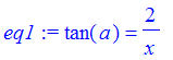
>	eq2 := tan(a)=3/(5-x);

>	sol := solve({eq1,eq2},{a,x});

So the player should bounce the ball off at a 45 degree angle.  This is the way most contrived problems work out.  If we were to jiggle the distance of the cue ball from the edge a little, we would expect the angle to jiggle too.  That is where parameterization comes into play.   We could parameterize this problem in several ways.  For example, replace the distance of the cue ball from the edge with a parameter h  and rework the problem.

>

>	eq1 := tan(a)=h/x;

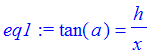
>	eq2 := tan(a)=3/(5-x);

>	sol := solve({eq1,eq2},{a,x});

>

Now we can investigate questions such as:

Question: What happens to the angle as the cue ball moves away from the edge?  towards the edge?

A Solution: The ball moves away from the edge as h gets larger.  By looking at the expression for a in terms for h, we see that the angle gets closer to 90 degrees.  On the other hand as h gets closer to 0 (as the ball moves towards the edge) the angle gets closer to arctan(3/5), or

>	evalf(180/Pi*arctan(3/5));

degrees.

Exercise:  Define a word  drawbounce := proc(h) which takes h, the distance of the cue ball from the edge and returns a picture of the cue ball, the red ball and the path the cue ball takes if it bounces once off the lower edge of the table.  Leave all the other data the same as given in the original problem.

Exercise:  Use the word drawbounce to make a movie of what happens to the path of the cue ball as the  cueball starts from a point closer to the edge of the table.

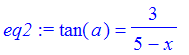
Exercise:    Suppose  that the edge of the billiard table opposite the x-axis is 4 feet wide and the player wants to bounce the cue ball twice before it hits the red ball. What angle should he bounce it off the edge?  

Solution.

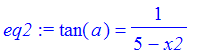
The  second edge has equation     , and the second bounce point will be  (x2,4).  Notice that the angle of reflection of the first bounce equals the angle of incidence of the second bounce, since the two edges are parallel.  So we have three ways two express the angle a in terms of  x and x2.

>

>	eq1 := tan(a)=2/x;

>	eq2 := tan(a)=1/(5-x2);

>	eq3 := tan(a)=4/(x2-x);

>

Now solve the equations for x,x2, and a.

>	solve({eq1,eq2,eq3},{x,x2,a});

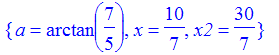
>	evalf(convert(arctan(7/5),degrees));

>

So  the player should bounce the ball off at about a 54.5 degree angle. Comparing this with the first problem, we note that the bounce angle should be larger than 45 degrees since the player must bounce the ball twice.  

Exercise:   What is the angle if the cue bounces off the edge     first?

Problem:  Suppose you are standing at the point (0,0,4) on the z-axis, looking  down towards the x-axis.  A spherical water tank 2 units in diameter is centered on the origin (0,0,0).    You can't 'see' the points on the x-axis close to (0,0,0) because the water tank is in the way, but you can see points far out on the x-axis. So, for example, the line connecting the point (10,0,0) to (0,0,4) doesn't touch the water tank (does it?), so you can 'see' that point.   The question is, what is the smallest point (a,0,0) on the positive x-axis you can see from (0,0,4).

Solution.

Let (c,0,d) be the point on the tank such that the line through (0,0,4) and (c,0,d) is tangent to the tank. So the triangle with vertices (0,0,0), (c,0,d), and (0,0,4) is a right triangle.   Using Pythagoras' theorem, this means that  

>	eq1 := c^2 + d^2 + c^2 + (d-4)^2 = 4^2;

>

 But also  

>	eq2 := c^2+d^2=1;

>

Since the three points [a,0,0], [c,0,d], and [0,0,4] are collinear,

>	eq3 := (d-0)/(c-a)=4/(-a);

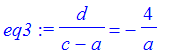
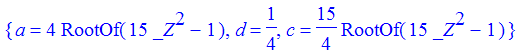
>	solve({eq1,eq2,eq3},{c,d,a});

>

By inspection, we see that      is the smallest positive real number the observer can see from (0,4).

We can draw a picture of the observer, the water tank, the line of sight from the observer to the x-axis.

>	tank := plot3d(1,theta=0..2*Pi,phi=0..Pi/2,coords=spherical):

>	lineofsight := plots[polygonplot3d]([[0,0,4],[4/sqrt(15),0,0]], thickness=2,color=black):

>	plots[display]([tank,lineofsight], scaling=constrained,axes=boxed);

Exercise:    Suppose you are at the point (0,0,h) on the z-axis looking toward  the positive x-axis.  What is the smallest point you can see on the positive x-axis?  Where are you if the smallest point  you can see is (10,0,0)?

Question:  What happens if we replace the  spherical tank with a parabolic cylinder, say     ?

Problem:  The foot of a ladder is placed at [3,0] and leaned up against a parabolic hill     .   Where does the ladder cross the y-axis?

Solution:

Draw a picture, showing the hill and the ladder.  Mark the point where the ladder crosses the y-axis [0,a].  Mark the point where the ladder touches the hill, .   The ladder is tangent to the hill at    .   We could figure out a if  we knew the slope of the ladder.   So take  a  point close to   ( )  on the hill.  Say the point is  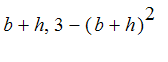 ( )  where h is a small number (but not zero).    The approximate slope of the ladder is the slope of the line through  these two points.  Calculate this slope, simplifying as much as possible.   Then find  the limiting value of this slope as h approaches 0, that is, as the   point   moves toward      on the parabola.  To find the slope using Maple,  

>	f := x -> 3 - x^2;

>	approxslope := (f(b+h) - f(b)) / ((b+h)  - b);

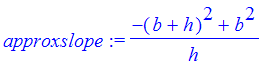
>	approxslope := simplify(approxslope);

>	slope1 := limit(approxslope,h=0);

But the slope of the ladder is also the slope of the line through   [3,0] and  .

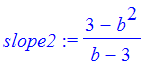
>	slope2 := (3-b^2)/(b-3);

>

   Now set these slopes equal and solve for b.

>	sol := solve(slope1=slope2,b) ;

    Which solution do we want?   It will have to be the smaller term (why?) After having decided that, find a by finding where the ladder crosses the y-axis.

>	b := min(sol);

>

>	ladder :=  x -> slope2*(x-b) + f(b);

>	a:= ladder(0);

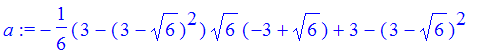
>	simplify(a);

>	evalf(a,4);

>	plot({f,ladder},0..3,color=black);

>

Problem:  A  5 foot ladder is leaning up against a parabolic hill    .    The foot of the  ladder is on the positive x-axis, and the top of the ladder is on the y-axis.  Describe the position of the ladder, by locating the coordinates of the foot of the ladder and the top of the ladder.     Note: This problem may have two different solutions.  Draw a picture and show how two positions may be possible.

Solution:

First define the hill.  The ladder leans up against the hill at the point [b,f(b)],
and will be tangent to the hill there.  By our calculations in the previous
problem, the slope of the ladder will be  at that point.

>

restart;

>	f := x->3-x^2;

>	slope := -2*b;

So we could  define the tangent line function at (b,f(b)).  That will be the ladder.

>	tang := x -> -2*b*(x-b)+ f(b);

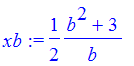
Then get the x and y intercepts of the ladder, call them xb and yb.

>	xb := solve(tang(x)=0,x);

>	yb := tang(0);

 The ladder is 5 feet long.  This gives us the equation we need to determine  the value of b.

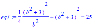
>	eq1 := xb^2+yb^2=5^2;

Let's manipulate this equation.

>	eq2 := expand(4*b^2*simplify(eq1));

>	eq3 := lhs(eq2)-rhs(eq2);

Now we are interested in finding the roots of eq3, where the graph of eq3 crosses the b axis.   So plot the graph.   First we graphed it over the interval 0..3, but then narrowed it down to the interval 0..1.7.  

>	plot(eq3,b=0..1.7);

Indeed, we can see by looking that there are two positions for the ladder, a high position and a low position.

>	sol := fsolve(eq3,b,0..1.5);

Now, to draw a picture, showing the hill and both positions of the ladder.

>	plot({f,subs(b=sol[1],op(tang)),

>	subs(b=sol[2],op(tang))},0..4,0..5,color=black);

>

Exercise:   In the ladder problem above, suppose we shorten the ladder.  We can imagine that as the ladder gets shorter, the two positions the ladder can occupy get closer to each other, until at last they coincide. What is the shortest ladder that can lean against the hill so that its foot is on the x-axis and its top is on the y-axis?

Solution:

 Go back to the ladder and look at the expression    .  This represents the square of the length of the ladder. What we can do is plot the square root of this expression over the interval 0..3 and find the low point on the graph.

>	plot(sqrt(xb^2+yb^2),b=0..3,y=0..20);

The shortest ladder is around  4.3 feet long.