
Early Integration.
At least as many problems can be solved using integration as can be solved using differentiation, so we need to find out about it too.
Integration involves adding up, which Maple does with sum .
Learning to use the Maple words Sum and sum .
Sum is the passive form of sum, so you can set up an equation displaying and computing the sum of the first 100 positive integers.
| > | Sum(i, i=1..100)=sum(i, i=1..100); |

| > |
Suppose we wanted to compute the sum of the arithmetic sequence
4 + 7 + 10 + 13 + .... + 301
First thing we need to figure out is the number of terms in this sum. Well, the common difference is 3 and the last term can be written as
![]() where
where
| > | i = (301-4)/3; |
![]()
So, there are 100 terms and we can sum this as
| > | Sum(4+i*3,i=0..99)=sum(4+i*3,i=0..99); |

Exercise: Find the sum of the square roots of i, as i goes from 1 to 10.
If we proceed as before,
| > | Sum(sqrt(i),i=1..10)=sum(sqrt(i),i=1..10); |

the sum is not computed. Use evalf to convert it to a decimal.
| > | Sum(sqrt(i),i=1..10)=evalf(sum(sqrt(i),i=1..10)); |

Exercise: Calculate the value of the following sum for n taking values 4, 8, 12 and n. What is the limiting value of the sum as n gets large?
| > | seq(Sum((1/2)^i,i=0..4*j)=sum((1/2)^i,i=0..4*j),j=1..3); |

| > |
| > | Sum((1/2)^i,i=0..n)=sum((1/2)^i,i=0..n); |

| > |
| > |
As n gets large,
 goes to 0, so the whole sum goes to 2.
| > | Sum((1/2)^i,i=0..infinity) =limit(Sum((1/2)^i,i=0..n),n=infinity); |

| > |
Riemann Sums with the student package
There are some useful words in the student package dealing with integration.
| > | with(student); |
![]()
![]()
![]()
For example, middlesum and middlebox compute and display a regular Riemann sum where the mark is chosen as the midpoint in each subinterval. For example, to get the middle regular Riemann sum for x^2 from 0 to 1 with 10 subintervals,
| > | middlesum(x^2,x=0..1,10) = value(middlesum(x^2,x=0..1,10)); |

| > | middlebox(x^2,x=0..1,10); |
![[Maple Plot]](images/hand715.gif)
| > |
Two Area Problems
Exercise: Plot the ellipse
 with a parametric plot. Estimate the area of the ellipse. Use the fact that it is four times the area under the graph of
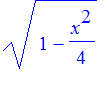 for x between 0 and 2.
Solution:
A
parameterization of the ellipse
is to let
![]() , as t goes from 0 to
, as t goes from 0 to
![]() .
.
| > | ellipse := [2*cos(t),sin(t),t=0..2*Pi]; |
![]()
| > | plot(ellipse,scaling=CONSTRAINED); |
![[Maple Plot]](images/hand721.gif)
The upper ellipse is the graph of the function
| > | f := x -> sqrt(1- x^2/4); |

| > |
We can use leftsum and rightsum to estimate the area.
| > | for i from 1 to 5 do left := 4*evalf(value(leftsum(f(x),x=0..2,25*i))); right := 4*evalf(value(rightsum(f(x),x=0..2,25*i))); print(left,right,right-left); od: |
![]()
![]()
![]()
![]()
![]()
By inspecting the table of numbers, we see that area is between 6.24 and 6.31.
| > |
Exercise: For the function
 , plot the function and determine the region R where the graph of f lies above the x-axis. Make the sketch of R and compute the endpoints of the base of R. Use
student[middlesum]
to find the area of the region R to within 0.1.
Solution:
First plot the function and calculate the endpoints of R.
| > | y := 10 - x^4 + 10*x; |
![]()
| > | plot(y,x=-2..3); |
![[Maple Plot]](images/hand730.gif)
| > | sol := fsolve(y,x); |
![]()
| > | for i from 1 to 5 do value(student[middlesum](y,x=sol[1]..sol[2],20*i)) od; |
![]()
![]()
![]()
![]()
![]()
The area looks to be 41.7 to the nearest 0.1, using middlesum with 100 subdivisions.
The fundamental theorem of calculus tells us that a definite integral of a continuous function f can be evaluated by first finding an antiderivative of f and then calculating the difference of its values at the endpoints: In symbols,
 provided
 .
.
You can use the Maple word int to find antiderivatives, (aka indefinite integrals).
For example, to find an antiderivative of
 , use int.
| > | Int(x^2 + cos(x/5),x)=int(x^2 + cos(x/5),x); |

Notice that there is a passive form of int, Int , for typesetting purposes.
You can also use int to evaluate definite integrals. For example, if we want to plot the region under the graph of
 for x between 0 and 2 and calculate its area.
| > | restart; |
| > | f := x-> x^2 + cos(x/5); |

| > | Int(f(x),x=0..2)=int(f(x),x=0..2); |
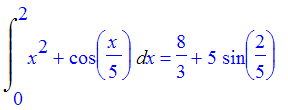
| > | area := evalf(int(f(x),x=0..2)); |
![]()
| > |
We will use plots[polygonplot] to shade the region.
| > | ### WARNING: semantics of type `string` have changed plots[polygonplot]( [ [2,0],[0,0],[0,f(0)],seq([x/10,f(x/10)] , x=0..20) ],color=gray,title= cat(`Area = `,convert(area,string)) ); |
![[Maple Plot]](images/hand745.gif)
| > |
Exercises:
Exercise: For each of the functions below, Sketch the region under the graph and calculate the area of the region using the fundamental theorem of calculus.
a)
 , for
, for
![]()
| > |
| > |
b) Under the arch of
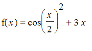 which contains x=0. .
| > |
| > |
c) f(x) = piecewise( x<1, sqrt(x) ,x>=1,x^2); for x between 0 and 2.
![x^2+cos(1/5*x) = PIECEWISE([x^(1/2), x < 1],[x^2, 1 <= x])](images/hand749.gif)
| > |
| > |
Suppose you picked at random 1000 numbers between 0 and 1. What would you expect the average of the squares of these numbers to be, about?
Solution .
First let's look up how rand works.
| > | ?rand |
So to get a function which returns random numbers between 0 and 1, we could do something like this:
| > | f := rand(10^7)/10.^7: |
| > | f(); |
![]()
| > | s := 0: for i from 1 to 1000 do s := s+f()^2 od: s/1000; |
![]()
| > |
Looks like its around a third.
On the other hand, you could estimate the average value by averaging the values at n equally spaced points in the interval. Here is a procedure for doing this. The inputs are f, the function to be averaged; a,b, the endpoints of the interval where the function is evaluated; and n, the number of equally spaced values to be averaged.
| > | av := proc(f,a,b,n) local i,dx; dx := (b-a)/n; evalf(sum(f(a+i*dx),i=1..n)/n); end: |
| > |
So to estimate the average value of x^2 as x ranges from 0 to 1, we could generate a sequence of estimates
| > | for i by 100 from 100 to 400 do print(i, av(x->x^2,0,1,i)) od; |
![]()
![]()
![]()
![]()
This seems to give about 1/3 also.
The last estimate can be turned into a regular Riemann sum. Let
 denote the length of each subinterval in the regular partition of [a,b] into n subintervals. Then the average and Riemann sum are the same:
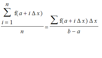
As n gets large, this Riemann sum converges to the integral of the function over the interval divided by the length of the interval. Thus we are justified in defining the average value as an integral.
Problems.
Exercise: The temperature in the 24 period from 0..24 is given as
 . Find the average temperature over the time interval. Find a time t when it is the average temperature. Also find the maximum temperature and minimum temperature.
| > |
| > |
Exercise: Suppose f is a continuous function on [a,b], with average value T. Show that there is an x in [a,b] so that f(x) = T.
| > |
| > |
Modeling the flow of air in lungs:
The rate of change of the volume of air in the lungs can be modeled very roughly (according to some texts) by the function
| > | f := t -> 1/2*sin(2*Pi*t/5); |

| > |
| > |
where volume is measured in liters and time is measured in seconds. So the actual volume of air in the lungs would obtained by integrating f. Here we are assuming there is no air in the lungs at time 0.
| > | Int(f(tau),tau=0..t) = int(f(tau),tau=0..t); |

| > | F := unapply(int(f(tau),tau=0..t),t); |

Let's plot the rate of airflow and the volume function to get a feel for their behavior.
| > | plot({f,F},0..10); |
![[Maple Plot]](images/hand762.gif)
| > |
Questions.
Question: Which is the rate of airflow function and which is its integral?
Question: What is the maximum volume of air in the lungs in this model? The minimum volume?
Question: When are the lungs half-full?
Question: What is the average rate of airflow in the lungs over the time interval [0,2.5]? [2.5,5]? [0,5]?
| > | ar := evalf(int(f(t),t=0..2.5)/2.5); |
![]()
| > |
About .32 liters per second on average.
Question: What is the average volume of air in the lungs over the time interval [0,2.5]? [0,5]?
| > | av := evalf(int(F(t),t=0..2.5)/2.5); |
![]()
| > |
About .4 liter air in the lungs on average.
Actually, there are different, perhaps more realistic models of the rate of airflow into the lungs. For example, consider this one,
| > | g := t -> (3/8-1/4*cos(4*Pi*t/5))*sin(2*Pi*t/5); |

| > |
Problem: Using the function g to model the rate of airflow in the lungs, find the volume G of air in the lungs at time t. (Assume as before that G(0) = 0.) Plot both g and G over the time interval [0,10]. Describe qualitatively a difference that you note between this model and the model we looked at above. Calculate the maximum rate of airflow in this model. What is the maximum volume of air in the lungs in this model? What is the average volume of air in the tank in the time interval [0,5]
Exercise: Find the upside down parabola
 so that the area between it and the parabola
 is 100. Draw a diagram.
Solution.
Set up the functions which bound the region.
| > | restart; |
| > | f := x -> a-x^2; |
![]()
| > | g := x-> x^2; |
![]()
| > |
Find the points where the functions cross.
| > | sol := solve(f(x)=g(x),x); |

| > |
Get the area of the region. By inspection, we see that sol[2] is the left endpoint where the functions cross.
| > | area := int(a-2*x^2,x=sol[2]..sol[1]); |
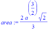
| > | sol; |

Solve an equation.
| > | sol2 := fsolve(area=100,{a}); |
![]()
| > | assign(sol2); |
| > | plot({f ,g }, sol[2]..sol[1]); |
![[Maple Plot]](images/hand774.gif)
| > |
Another area problem: The parabola
 is tangent to the graph of
![]() at two points and the area of the region bounded by their graphs is 10. Find a, b, and c. Make a sketch.
at two points and the area of the region bounded by their graphs is 10. Find a, b, and c. Make a sketch.
Solution :
The axis of the parabola is
 . That is also the axis of
![]() , so
, so
 , or
, or
![]() . The point where the slope of the parabola is 1 is on both graphs. Call the point [x0,y0]. Then
. The point where the slope of the parabola is 1 is on both graphs. Call the point [x0,y0]. Then
 and
and
![]() .
.
| > | restart; |
| > | eq1 := x0-1 = a*x0^2 -6*a*x0 + c; |
![]()
| > | eq2 := 1 = 2*a*x0 - 6*a; |
![]()
| > | ac := solve({eq1,eq2},{a,c}); |

| > |
Finally, the area between the curves is 100, so the righthand half is 50.
| > | eq3 := Int (a*x^2-6*a*x+c-(2+x-3),x=3..x0)=50; |

Integrating,.
| > | eq3 :=int(a*x^2-6*a*x+c-(2+x-3),x=3..x0)=50; |
Sollving for x0
| > | sol :=solve(subs(ac,eq3),x0); |
![]()
| > | assign({x0=sol[1]}); assign(ac); |
| > | plot({2+abs(x-3),a*x^2-6*a*x+c}, x=sol[2]-2..sol[1]+2,color=black); |
| > |
| > |