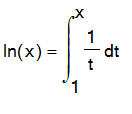
 , came along later. The key fact is that this area grows arithmetically as x grows geometrically.
A Useful Function -- The natural logarithm
The logarithm function was first introduced in the early 1600's by John Napier to reduce the toil of performing multiplication and division of numbers. The idea was quickly accepted worldwide.
Napier's logarithm was defined differently from the way it would be now. The idea of defining the logarithm of x for x > 0 to be the signed area under the curve 1/x, that is,
, came along later. The key fact is that this area grows arithmetically as x grows geometrically.
Problem
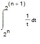
: Consider the sequence of powers of 2,
![a[n] = 2^n](images/hand82.gif) , n = 1, 2, .... This is a
geometric sequence
, that is, the ratio of consecutive terms is constant (in this case, the common ratio is 2). Now let
, n = 1, 2, .... This is a
geometric sequence
, that is, the ratio of consecutive terms is constant (in this case, the common ratio is 2). Now let
![b[n] = Int(1/t,t = 1 .. a[n])](images/hand83.gif) , for n = 1, 2 .. We claim that the sequence
, for n = 1, 2 .. We claim that the sequence
![]() is an
arithmetic sequence
, that is, the difference of consecutive terms is constant. To compute the difference, first use the definition:
is an
arithmetic sequence
, that is, the difference of consecutive terms is constant. To compute the difference, first use the definition:
![b[n+1]-b[n] = Int(1/t,t = 1 .. 2^(n+1))-Int(1/t,t = 1 .. 2^n)](images/hand85.gif) . This difference of integrals can be written as the single integral
. This difference of integrals can be written as the single integral
 . But now make the substitution
 into the integral. Then
 and the integral becomes
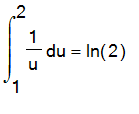 . It follows from this that
![]() , an arithmetic sequence as we claimed above.
, an arithmetic sequence as we claimed above.
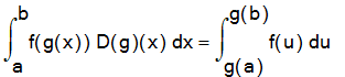
Exercise: Use the change of variable formula, given below, to establish other properties of the natural logarithm, such as i)
![]() , for all positive x and y, and ii)
, for all positive x and y, and ii)
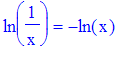 , for all x > 0.
| > |
| > |
Exercise: Use a sequence of student[rightsum]'s to estimate
![]() by Riemann sums to 4 decimal places.
by Riemann sums to 4 decimal places.
| > |
| > |
Exercise: Which line
![]() divides the region under the graph of
divides the region under the graph of
 between 1 and 2 into two regions with equal area? Sketch the graphs.
Solution:
First find where the line crosses 1/x.
| > | y := m*(x-1); |
![]()
| > | b := solve(y=1/x,x); |
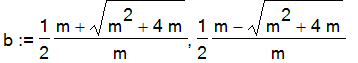
We want the first solution. That's the one that crosses the right branch of 1/x. The equation we want to solve then is:
| > | eq := Int(1/x-y,x=1..b[1])=1/2*ln(2); |
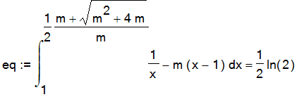
| > | m := fsolve(value(eq),m); |
![]()
Now go ahead and draw the picture to see if it looks about right.
| > | plot({1/x,y,[[2,0],[2,1/2]]},x=1..2,scaling = constrained,color=black); |
![[Maple Plot]](images/hand821.gif)
This looks to be cut in half.
Exercise: Find the parabola
 which is tangent to the graph of
![]() . Sketch the graph.
. Sketch the graph.
Solution:
Let [x1,ln(x1)] be the point of tangency. Then ln(x1) is equal to x1^2 + b. That's the first equation.
| > | restart; eq1 := x1^2+b = ln(x1); |
![]()
But also the derivative of x^2 + b at x1 and 1/x at x1 must be equal. Thats the second equation, which should be enough to determine x1 and b.
| > | eq2 := 2*x1 = 1/x1; |
![]()
| > | sol := solve({eq1,eq2},{x1,b}); |
![]()
There seem to be two values for x1, 1/sqrt(2) and -1/sqrt(2). But the ln is not defined at -1/sqrt(2) so x1 is the first one.
| > | x1 := 1/sqrt(2); |
![]()
| > | b := ln(x1)-1/2; |
![]()
| > | plot({ln(x),x^2+b},x=-2..2,thickness=2); |
![[Maple Plot]](images/hand829.gif)
| > |
Exercise: Find the parabola
 which is tangent to the graph of
 . Sketch the graphs.
| > |
| > |
Exercise: Find the local extreme values of
![]() . Sketch the graph.
. Sketch the graph.
| > |
| > |
Exercise: Sketch the region bounded by
 and
and
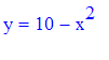 . Find the area of the region.
| > |
| > |
8. The line
![]() and the graph of
and the graph of
 bound a region of area 10. Find m and plot the graphs.
| > |
| > |
Exercise: The line
![]() does not intersect the graph of
does not intersect the graph of
![]() . (Does it?) Find the point on the line which is closest to the graph. Sketch the graphs.
. (Does it?) Find the point on the line which is closest to the graph. Sketch the graphs.
Solution:
First look at the graphs.
| > | line := 2*x+1; |
![]()
| > | lnln := ln(ln(x)); |
![]()
| > | plot( {line,lnln} ,x=-5..5,thickness=2); |
![[Maple Plot]](images/hand841.gif)
| > |
Clearly they don't intersect. The lnln function is only defined for x > 1 and is concave down, so it will never cross the line. The closest point looks to be near x=1.5 It would be the point on the graph where the tangent line is parallel with the given line. So it would be where the derivative is 2.
| > | x1:=fsolve(diff(lnln,x)=2,x,1..1.5); |
![]()
| > | plot({line,lnln,-1/2*(x-x1)+subs(x=x1,lnln)},x=-5..5,scaling=constrained,thickness=2,color=black); |
![[Maple Plot]](images/hand843.gif)
| > |
The inverse of the natural log
The inverse of the natural logarithm is called the exponential function .
It is predefined in Maple as
exp
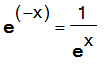
. It is called the exponential function because it obeys the 'laws of exponents',
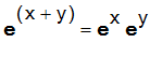 and
and
 . In this setting, e is defined to be the number such that
![]() . This says that exp(1)=e. So, exp(2) = exp(1+1) = exp(1)*exp(1) = e^2 . Also, exp(1/2) = e^(1/2) , since exp(1/2)^2 = exp(1/2)*exp(1/2) = exp(1/2 + 1/2) = e . With some work, you can show that exp(x) = e^x for any rational number x, and so it is compatible to define e^x = exp(x) for all real numbers x.
. This says that exp(1)=e. So, exp(2) = exp(1+1) = exp(1)*exp(1) = e^2 . Also, exp(1/2) = e^(1/2) , since exp(1/2)^2 = exp(1/2)*exp(1/2) = exp(1/2 + 1/2) = e . With some work, you can show that exp(x) = e^x for any rational number x, and so it is compatible to define e^x = exp(x) for all real numbers x.
The number e can also be shown to be the limit of
 as n gets large. We can check this out numerically by defining a function which takes as input a positive integer n and outputs the decimal value of the nth term of the sequence.
Exercise: By experimenting, find the smallest value of n which gives e correct to 5 significant digits.
| > | approxe := n -> evalf((1+1/n)^n); |
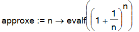
| > | approxe(100); |
![]()
| > |
The exponential function rises more quickly than any polynomial function.
The linear function which has the same value and same derivative as the exponential function y = exp(x) at x = 0 is the tangent line y = x + 1 at x=0. The quadratic function that has the same value, and first and second derivatives as exp(x) at x = 0 is the quadratic function 1 + x + (1/2)x^2 . Continuing, the polynomial of degree n which has the same value and first n derivatives as the exponential function can be shown to be
 . We can plot any number of these on the same graph with exp(x).
| > | efun := plot(exp,-1..4,color=black,thickness=2): |
| > | pfuns := plot({1+x,1+x+1/2*x^2,1+x+x^2/2+x^3/3!, 1+x+x^2/2+x^3/3!+x^4/4!,1+x+x^2/2+x^3/3!+x^4/4!+x^5/5! },x=-1..4,color=tan): |
| > | plots[display]([efun,pfuns]); |
![[Maple Plot]](images/hand851.gif)
As can be seen from the plots, the polynomials get closer to the exponential function but not rise as fast. These polynomials are the Taylor approximating polynomials for the exponential function, and can be formed for any function which has derivatives of all orders.
The functions y = x^2 and y = 2^x cross each other 3 times. Find
two of the points of intersection by inspection of the equation x^2 = 2^x . Then plot the two functions on the same graph and estimate, from the graph, the coordinates of the third point.
The exponential and logarithm functions can be used to define the other exponential functions
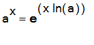 , so long as a is positive.
| > |
Exercise: The functions
![]() and
and
![]() touch each other 2 times. Find one of the point of intersection by inspection of the equation
touch each other 2 times. Find one of the point of intersection by inspection of the equation
 . Then plot the two functions on the same graph and estimate, from the graph, the coordinates of the second point. Find the value of a between 2 and 3 such that
![]() and
and
![]() touch exactly once. Plot the resulting graphs.
touch exactly once. Plot the resulting graphs.
| > |
| > |
Two cups o' soup: Suppose that two cups of soup, the first at 90 C and the second at 100 C are put in a room where the temp is maintained at 20 C. The first cup cooled from 90 C to 60 C after 10 minutes, at which time the second cup is put in a freezer at -5 C. How much longer will it take the two cups to reach the same temperature?
Solution:
Assuming Newton's Law of cooling, we see that the first cup's temperature is given by
| > | restart; |
| > | f := t -> 20 + 70*exp(k*t); |
![]()
where k is determined by the information given that the first cup cools to 60 C in 10 minutes (i.e. solve the equation f(10)=60 for k).
| > | k := solve(f(10)=60,k); |
![]()
Assume that this value of k is also valid for the second cup. (Why shouldn't it be, they are both soup.) So the second cup's temperature is given by
| > | g := t -> 20 + 80*exp(k*t); |
![]()
| > |
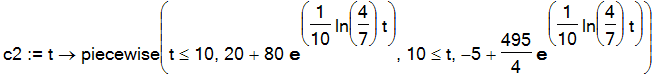
for the first 10 minutes. From that time on, the second cup's temperature is given by
| > | h := t -> -5 + (itemp - (-5))*exp(k*t); |
![]()
| > |
where itemp is the temperature that the 2nd cup would start at in order for it to cool to g(10) degrees C if it were in the freezer from the start. So itemp satisfies the equation
We can combine these two rules into one function using piecewise .
| > | c2 := unapply(piecewise(t<=10,g(t),t>=10, h(t)),t); |
| > |
| > | eq := -5 + (itemp +5)*exp(k*10) = g(10); |
![]()
| > |
Solving for itemp,
| > | itemp := solve(eq,itemp); |
![]()
| > |
Now plot the two temperature curves.
| > | cup1 := [t,f(t),t=0..20]; |
![cup1 := [t, 20+70*exp(1/10*ln(4/7)*t), t = 0 .. 20]](images/hand865.gif)
| > |
| > | cup2 := [t,c2(t),t=0..20]; |
![cup2 := [t, PIECEWISE([20+80*exp(1/10*ln(4/7)*t), t <= 10],[-5+495/4*exp(1/10*ln(4/7)*t), 10 <= t]), t = 0 .. 20]](images/hand866.gif)
| > | plot( {cup1,cup2},thickness=2 ); |
![[Maple Plot]](images/hand867.gif)
| > |
The cups are at the same temperature before another 5 minutes pass.
| > | etime := solve(f(t)=c2(t),t); |
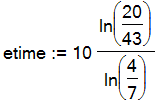
| > | evalf(etime),` minutes from time 0`; |
![]()
At that time the common temperature is
| > | f(etime)=evalf(f(etime)),` degrees`; |
![]()
Inverse Functions: The inverse trig functions
None of the trignometric functions are 1 to 1, however each can be restricted to a domain so that it is 1-1 on that domain and all values of the function are attained. For example, if we restrict the tangent function to the interval (-Pi/2 , Pi/2), it is 1-1 there. So the inverse tangent or arctan function is defined as the inverse of the restriction. The same sort of thing is done to define the arcsin and arcsec functions.
| > | Digits:=3: plots[display](matrix(1,3,[[plot(arctan ,-10..10,thickness=2), plot(arcsin ,-10..10 ,thickness=2), plot(arcsec ,-10..10,thickness=2)]])); Digits := 10: |
![[Maple Plot]](images/hand871.gif)
One thing which makes the inverse trig functions especially important is that they all have algebraic derivatives. So they play an important role in finding antiderivatives of functions.
| > | restart; |
| > | diff(arctan(x),x); |

| > | plot({arctan,D(arctan)},-5..5,thickness=2); |
![[Maple Plot]](images/hand873.gif)
Exercise: Find the critical points of
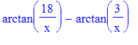 , for positive x. Make a sketch which shows any extreme values.
| > | y := arctan(18/x)-arctan(3/x); |
![]()
| > | plot(y,x=-20..20); |
![[Maple Plot]](images/hand876.gif)
By inspection, we can be pretty sure that y has a single max value at around [7,.8] and a symmetrically placed min at around [-7,-.8]. To be more specifiy
| > | extr :=solve(diff(y,x),{x}); |
![]()
| > |
There is a maximum at
![]() and a minimum at
and a minimum at
![]() .
.
Exercise: Bill, driving a red Mustang at 120 miles per hour, is headed straight toward a railroad crossing in Kansas. When he is a mile from the crossing he notices a train, coming towards the same intersection. He estimates the speed of the train to be 60 mph and the distance of the engine from the intersection to be a mile. The train looks to be about 300 yards long. Keeping his eye on the train during the next minute, he notices that the angle subtended at his eye by the train got larger at first and then began decreasing. How far was Bill from the intersection when the angle was maximum?
Solution:
First, draw a picture. Let's use yards, minutes, and degrees for units. Then Bill's distance from the intersection t minutes from the time Bill first saw the train was
![]() yards and the engine's distance was x = y yards. The distance of the caboose from the intersection is x + 300 yards. The angle subtended at Bills eye by the train is
yards and the engine's distance was x = y yards. The distance of the caboose from the intersection is x + 300 yards. The angle subtended at Bills eye by the train is
![]() Now
Now
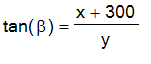 and
and
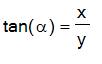 .
.
So the function to be maximized is
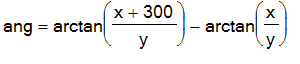 .
.
| > | restart; |
| > | ang := arctan((x+300)/y)-arctan(x/y); |
![]()
| > | y := 1762*(1-2*t); x:= 1762-1762*t; ang; |
![]()
![]()
![]()
| > | plot(ang,t=-2..3); |
![[Maple Plot]](images/hand889.gif)
| > |
The plot shows that there is a local maximum viewing angle before Bill gets to the crossing, and an absolute maximum after he crosses. To get the times, distances, and angles do the following:
| > | sol :=solve(diff(ang,t),t) ; |
![]()
| > | evalf([sol]); |
![]()
| > | asol :=evalf([seq(subs(t=sol[i],ang),i=1..2)]); |
![]()
| > | dsol :=evalf([seq(subs(t=sol[i],[x,y]),i=1..2)]); |
![]()
| > | evalf([seq(convert(asol[i],degrees),i=1..2)]); |
![]()
| > |
So Bill's view of the train is locally a maximum of about 5 degrees at about .24 minutes after he sees the train and about 912 yards before he crosses the intersection. His maximum view (about 13.5 degrees) of the train occurs at about .76 minutes and 912 yards beyond the crossing.
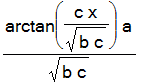
Exercise: Find an antiderivative for
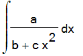
| > | int(a/(b+c*x^2),x); |
| > |
Exercise: Two hallways, meeting at right angles, have widths a and b. Find the width of the longest pole which can be slid around the corner.
| > |
| > |
Exercise: The bottom free corner of a page in a 8 inch by 6 inch book is folded back to the binding and creased so that the crease is as short as possible. What is measure of the angle formed by the crease at the bottom of the page?
| > |
| > |