 , then by make the change of variable
 we have a new, perhaps simpler integral
 , to work on.
Integration Techniques and Applications
You can use the student package in maple to practice your integration techniques. First load the student package by typing
| > | restart;with(student): |
Then read over the help screens on changevar , intparts , and value , paying particular attention to the examples at the bottom of the screens. Here are some examples.
Integration by substitution
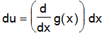
is based on the chain rule. Thus if we have an integral which looks like
, then by make the change of variable
![]() , and letting
we have a new, perhaps simpler integral
, to work on.
, and letting
we have a new, perhaps simpler integral
, to work on.
In Maple this is accomplished using the word changevar from the student package.
| > | assume(u::real,x::real); |
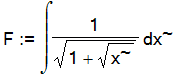
| > | F := Int(1/sqrt(1+sqrt(x)),x); |
| > |
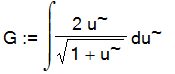
Let's try the change of variable sqrt(x) = u .
| > | G := changevar(sqrt(x)=u,F); |
| > |
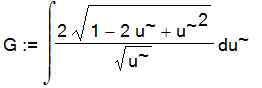
This does not seem to help. Lets try 1 + sqrt(x)= u
| > | G := changevar(1+sqrt(x)=u,F); |
| > |
Now we can do it by inspection, so just finish it off.
| > | G := value(G); |
![]()
| > |
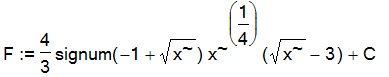
Now substitute back and add in the constant.
| > | F := subs(u=sqrt(x),G) + C; |
| > |
Integration by substitution is the method use try after you decide you can't find the antiderivative by inspection.
An Integration by Parts Problem:
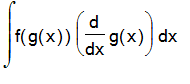
Integration by parts
is based on the product rule for derivatives. It is usually written
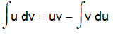 . It turns one integration problem into one which 'may' be more doable. Once you decide to use parts, the problem is what part of the integrand to let be u.
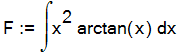
Integrate
| > | F := Int(x^2*arctan(x),x); |
| > |
The word is
intparts
. Let's try letting
 .
.
| > | G := intparts(F,x^2); |
| > |
That was a bad choice. Try letting
![]()
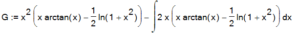
| > | G := intparts(F,arctan(x)); |

| > |
This is much more promising. Split off the integral on the end.
| > | H := op(2,G); |
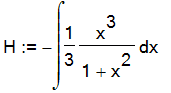
| > |
Now do a partial fractions decomposition of the integrand of H, using parfrac .
| > | H:= Int(convert(integrand(H),parfrac,x),x); |
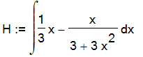
| > |
Now we can do it by inspection.
| > | H1 := 1/6*x^2 - 1/3*1/2*ln(1+x^2); |
![]()
| > |
Let's check this with the student value .
| > | simplify(value(H-H1)); |
![]()
| > |
Note the difference of a constant, which is fine for antiderivatives.
ETAIL : The problem of choosing which part of the integrand to assign to u can often be solved quickly by following the etail convention. If your integrand has an Exponential factor, choose that for u, otherwise if it has a Trigonometric factor, let that be u, otherwise choose an Algebraic factor for u, otherwise chose an Inverse trig function, and as a last resort choose u to be a logarithmic factor. Let dv be what's left over.
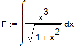
Find an antiderivative of
| > | F := Int(x^3/sqrt(x^2+1),x); |
| > |
The presence of
 suggests letting
![]() .
.
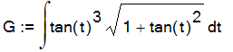
| > | G := changevar(x=tan(t),F,t); |
| > |
Now use the trig identity
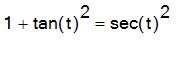 .
.
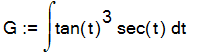
| > | G := subs(sqrt(1+tan(t)^2)=sec(t),G); |
| > |
Another substitution into the integrand.
| > | G := subs(tan(t)^3 = (sec(t)^2-1)*tan(t),G); |
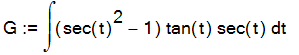
| > |
Let's make a change of variable,
| > | H := changevar(sec(t)=u,G); |
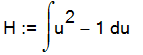
| > |
From here, we can do it by inspection.
| > | H := value(H); |
![]()
| > |
Now unwind the substitutions.
| > | G := subs(u=sec(t),H); |
![]()
| > | F := subs(t = arctan(x),G); |
![]()
| > | F := subs(sec(arctan(x))=sqrt(1+x^2),F) + C; |
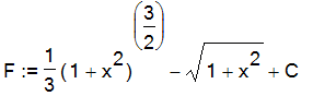
| > |
Checking this calculation:
| > | F1 := int(x^3/sqrt(x^2+1),x); |
![]()
| > |
It looks different, but is it?
| > | simplify(F-F1); |
![]()
| > |
Yes, but only by a constant.
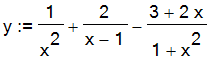
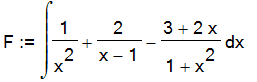
Integrate the rational function
| > | y :=(4*x^2+x -1 )/(x^2*(x-1)*(x^2+1)); |
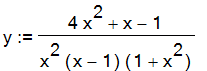
| > |
First get the partial fractions decomposition of y.
| > | y := convert(y,parfrac,x); |
| > |
We can almost do this by inspection, except for the last term.
| > | F := Int(y,x); |
| > | F := expand(F); |
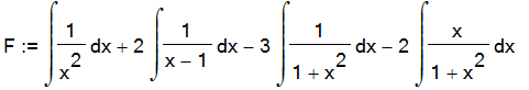
| > |
Now we can do each one by inspection. So we'll just use value .
| > | F := value(F) + C; |
![]()
| > |
Exercise:Use the student package to perform the following integrations.
| > |
| > |
| > |
| > |
| > |
| > |
![]()
| > |
| > |
| > |
| > |
| > |
| > |
![]()
| > |
| > |
Exercise: Find the area of the region enclosed by the x-axis and the curve
![]() on the interval
on the interval
![]() . Sketch the region. Then find the vertical line
. Sketch the region. Then find the vertical line
![]() that divides the region in half and plot it.
that divides the region in half and plot it.
| > |
| > |
Exercise: Find the length of the graph of the parabola
 from O(0,0) to P(10,100). Find the point
 on the graph which is 10 units from O along the graph. Make a sketch, showing the points O, P, and Q on the graph.
| > |
| > |
Exercise: Find the volume of the solid of revolution obtained by revolving the region trapped between the the graph of
 on
on
![]() and the x-axis about the x-axis. Sketch a graph. Does this volume approach a finite limit as n gets large?
and the x-axis about the x-axis. Sketch a graph. Does this volume approach a finite limit as n gets large?
| > |
| > |
Numerical Integration Problems
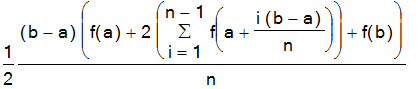
If you have a definite integral that you need to evaluate to a certain accuracy, one can always use a numerical integration formula or "rule", such as the trapezoid rule or Simpson's rule. The student package contains words for these two rules. And you may have already discovered on your own that when evalf(int(f(x),x=a..b); is entered, a numerical method is used to calculate an approximation.
The trapezoid rule is named for the way it approximates an integral by adding the signed areas of a number of trapezoids. The trapezpoid rule is already defined in the student package;
| > | student[trapezoid](f(x),x=a..b,n) ; |
Exercise: Derive the trapezoid rule directly from the definition of the area of a trapezoid as
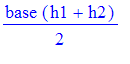 , where h1 and h2 are the heights of the trapezoid.
Here is a Maple procedure which draws a picture of the trapezpoids used to approximate the integral.
| > | drawtrap := proc(f,a,b,n) local dx,div, traps,i,tn,nn,ai,aim1,fai,faim1,clr; if n > 50 then RETURN(`Too many subdivisions..`) fi; dx := evalf((b-a)/n); div := (a,dx,i) -> evalf(a+i*dx); traps := plot(f,a..b,thickness=2,color=black): for i from 1 to n do aim1 := div(a,dx,i-1); ai := div(a,dx,i); faim1 := evalf(f(aim1)); fai := evalf(f(ai)): clr := tan; if faim1*fai <= 0 then clr := yellow fi; if faim1 <= 0 and fai <= 0 then clr := aquamarine fi; traps := traps, plots[polygonplot]([[aim1,0], [ai,0],[ai,fai], [aim1,faim1]], color=clr) od; tn := evalf(student[trapezoid](f(x),x=a..b,n)); ### WARNING: semantics of type `string` have changed tn := convert(tn,string); ### WARNING: semantics of type `string` have changed nn := convert(n,string); plots[display]([traps], title=cat(`T`,nn,` = ` ,tn)); end: |
| > | drawtrap(sin,0,3*Pi,8); |
![[Maple Plot]](images/hand955.gif)
Problem
. Use student[trapezoid] to estimate
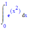 with 10 through 50 subdivisions.
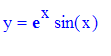
| > | for i from 1 to 5 do evalf(student[trapezoid](exp(x^2),x=0..1,10*i)) od; |
![]()
![]()
![]()
![]()
![]()
| > |
By looking at this sequence, we would feel fairly confident, (but not absolutely certain) that the value of the integral is between 1.46 and 1.47 There is a theorem which gives a bound on the error in the trapezoid rule .
Theorem. If there is a positive number
![]() such that
such that
![abs(diff(f(x),x) <= K[1])](images/hand963.gif) for all x in [a,b], then the actual error
for all x in [a,b], then the actual error
![abs(Int(f(x),x = a .. b)-trap[n])](images/hand964.gif) is no more than
is no more than
![K[1]*(b-a)^2/(2*n)](images/hand965.gif) .
.
Now the derivative of
 is
is
 . and clearly the maximum of the derivative on [0,1] is at x=1, so we can take
![]() . In order for the actual error in using the nth trapezoid rule to estimate the integral above to be less than .01 say, the theorem guarantees that if n is chosen large enough to satisfy the inequality
. In order for the actual error in using the nth trapezoid rule to estimate the integral above to be less than .01 say, the theorem guarantees that if n is chosen large enough to satisfy the inequality
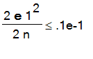 . Solving this,
| > | solve(2*exp(1)*1^2/(2*n) <= 1/100,n); |
![]()
| > | evalf(100*exp(1)); |
![]()
we see that taking n = 272 will suffice, although this is much too conservative, as we can see from our calculations with trapezoid above.
Exercise: Use the theorem find a value for n so that if
 is estimated with the trapezoid rule with n subdivisions, the estimate is within 1/1000 of the correct value. Use trapezoid to see if the estimate is conservative.
| > |
| > |
Simpson's rule is named for it's discoverer, Thos. Simpson, in the early 1700's. It is obtained by interpolating a quadratic through the endpoints and midpoint of the function and using the integral of the quadratic to estimate the integral of the function. So if the quadratic function is called quad, then quad(a) = f(a), quad(b)=f(b) and quad((a+b)/2)=f((a+b)/2). Using this, we can see that quad looks like
| > | restart; |
| > | quad := x->f(a) + (f(b)-f(a))/(b-a)*(x-a) + d*(x-a)*(x-b); |
![]()
and we can determine d by solving the equation
| > | eq := quad((a+b)/2)= f((a+b)/2); |
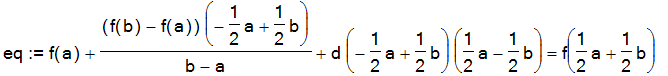
| > | d :=solve(eq,d); |
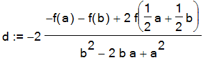
| > | quad(x); |
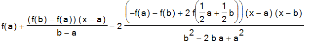
| > | int(quad(x),x=a..b); |
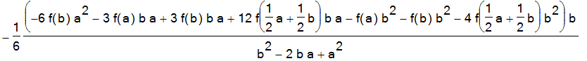
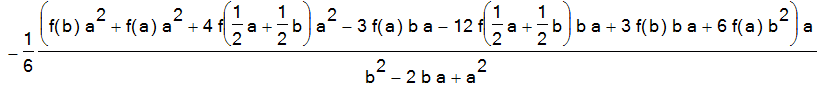
Now simplify this and factor the result of that
| > | simplify(%); |
![]()
| > | factor(%); |
![]()
| > |
| > |
Voila ! Simpson's rule. with two subintervals. Simpson's rule with an even number n of subintervals is defined in the student package.
| > | for i from 1 to 5 do evalf(student[simpson](exp(x^2),x=0..1,10*i)) od; |
![]()
![]()
![]()
![]()
![]()
We can see that Simpson's rule converges much more quickly on this integral than the trapezoid rule did above. There is a theorem which govern's the error in Simpson's rule.
Theorem: If you can find a positive number
![]() such that
such that
![abs(diff(f(x),x,x,x,x) <= K[4])](images/hand987.gif) for all x in [a,b], then the actual error
for all x in [a,b], then the actual error
![abs(Int(f(x),x = a .. b)-S[n])](images/hand988.gif) is no more than
is no more than
![K[4]*(b-a)^5/(180*n^4)](images/hand989.gif) .
.
We can apply this theorem to find out how large n must be taken so that the error in using Simpson's rule to estimate
 is no more than 1/100. The fourth derivative is
| > | diff(exp(x^2),x,x,x,x); |
![]()
This is maximum at x=1, so we can take
![]() . Now solve the inequality for n .
. Now solve the inequality for n .
| > | solve(76*exp(1)*1^5/(180*n^4)<= 1/100,n) ; |
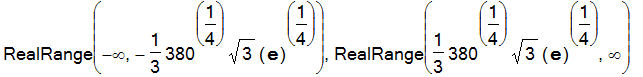
We can take n to be any even integer no smaller than
| > | evalf(1/3*380^(1/4)*3^(1/2)*exp(1)^(1/4)); |
![]()
so this is much better than the previous bound we got with the trapezoid rule.
We can check this prediction of '4 subintervals suffice' by using evalf(int) to compute the value correct to 10 digits and using this as the true value.
| > | truevalue := evalf(int(exp(x^2),x=0..1)); |
![]()
| > | approxvalue := evalf(student[simpson](exp(x^2),x=0..1,4)); |
![]()
| > | approxvalue - truevalue; |
![]()
So we see that the theorem predicted correctly. Whew!
Exercise: Use the theorem find a value for n so that if
 is estimated with Simpson's rule with n subdivisions, the estimate is within 1/1000 of the correct value. Use student[simpson] to see if the estimate is conservative. Also use evalf(int to check that the value of n predicted by the theorem is large enough.
More problems with Trapezoid and Simpson
Problem: If you apply Simpson's rule with only two subintervals to any cubic function, you will get the exact answer every time. Verify this assertion for the cubic
 . Prove the assertion, using the theorem giving the error bound on Simpson's rule.
Problem: Use the error bound on Simpson's rule above to estimate the error in using Simpson's rule with 6 subintervals to approximate ln(3). Use evalf(int to compute the truevalue and verify that the estimate on the error is not smaller than the actual error.
Solution:
First, define the function and take its 4th derivative.
| > | f := x -> 1/x; |
![]()
| > | f4 := diff(f(x),x,x,x,x); |

The 4th derivative is clearly maximum on the left hand endpoint of the interval [1,3], so
| > | K[4] := 24; |
![]()
| > |
The bound on the error given by the theorem is
| > | sbound := K[4]*(3-1)^5/(180*6.^4); |
![]()
So the error is less than 5 thousandths.
| > |
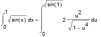
Exercise: The integral
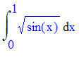 is difficult to estimate to within 1/1000 using the trapezoid rule or Simpson's rule. For one thing, the error bound theorems don't apply. Why? But if we we make the change of variable sqrt(sin(x)) = u , then we get a new integral to which the error bounding theorems apply. Why? How many subdivisions using Simpson do you need to estimate the new integral to within 1/1000? This exercise shows that the method of substitution is useful in numerical integration as well as symbolic integration
| > | Int(sqrt(sin(x)),x=0..1) = student[changevar](sqrt(sin(x))=u,Int(sqrt(sin(x)),x=0..1)); |