seqser.html

Sequences and Series

We have used sequences lots of times before. The sequence of estimates to the solution of an equation generated by Newton's Method is one. The sequence of estimates to the integral of a function over an interval obtained by subdividing the interval into more and more subintervals is another. These are examples of potentially infinite sequences. Theses are sequences we hope converge to the answer we seek, whether it be the solution of an equation or the value of an integral.

Formally, a sequence of numbers is defined as a function f whose domain is the positive integers. The terms of the sequence are the values of the function. So for example the 10th term of the sequence f is f(10).

A sequence f converges to a limit L if each interval containing L contains all but finitely many terms of the sequence. In this case, we would write .

The Maple word limit can be used to calculate many limits of sequences in a painfree manner. For example,

> limit((1+1/n)^n,n=infinity);

The next theorems summarize many of the properties of convergent sequences.

Theorem: If is an increasing sequence (ie, for all ), then converges if there is an upper bound on the terms of .

Theorem: If converges to and converges to , then converges to , converges to , and converges to . Also, if , then converges to .

Theorem: If is a sequence of positive numbers and is a sequence which converges to 0, then if for all , then converges to 0.

Theorem: If is continuous at , and is a sequence converging to , then the sequence converges to .

>

Periodic Points of functions.

Let f be a function, and let a be a point in the domain of f. If each value of f is in the domain of f, we can generate the sequence of iterates of a under f as follows: , , and in general for each positive integer n. If n is a positive integer such that , but for for all positive integers i < n, then a is called a periodic point of period n for f.

Period one points are called fixed points . You can locate the fixed points of a function by looking to see where the graphs of and cross. For example, the cosine function has one fixed point, as we can see by plotting.

> plot({cos(x),x},x=-Pi..Pi);

>

To find the fixed point more precisely, use fsolve .

> fix := fsolve(cos(x)=x,x,0..Pi);

>

An attracting fixed point is a fixed point a with the property that for points b close to a,

> limit(b[n],n=infinity) = a;

>

where , and for ...

A repelling fixed point is a fixed point a with the property that for points b close (but not equal) to a,

> limit(b[n],n=infinity) <> a;

>

where , and for , ... .

Here is a simple procedure to investigate periodic points and fixed points of a function.

>    iterate := proc(f,n,x)
    local a,i,s;
    a := evalf(x);
    s := a;
    for i to n do a := f(a);
    s := s,a od
    end:

>

For example, to investigate whether the fixed point of the cosine function is attracting or not, we can iterate the function at a point near the fixed point. Using the fixed point of the cos function,

> fix := fsolve(cos(x)=x,x);

> iterate(cos,10,fix-1),fix;

>

The fixed point seems to be an attracting one. On the other hand if we look at the fixed points of 2x(1-x),

> f := x-> 2*x*(1-x);

> fix := fsolve(f(x)=x,x);

> iterate(f,10,fix[1]-.2);

> iterate(f,10,fix[1]+.1);

> iterate(f,10,fix[2]+.4);

It seems that 0 is an repelling fixed point and that .5 is an attracting fixed point. Let's define a visual word to go with iterate. We have added a domain and range to allow you to determine the viewing window.

>

>    viterate := proc(f,n,start,domain,range)
     local a, i, s, gra, gpl, fpl, ipl;
    a := evalf(start);
    gra := [a,f(a)];
    for i to n do a := f(a);
    gra := gra,[a,a],[a,f(a)];
    od:
    gpl := plot([gra],color=red);
    fpl := plot(f,domain,color=black);
    ipl := plot(x->x,domain,color=blue);
    print(plots[display]([gpl,fpl,ipl],view=[domain,range]));
    end:

> viterate(x->2*x*(1-x),10,.8,-1..1 ,-1..1);

This gives a nice visual tool to investigate fixed points and periodic points of functions.

>

Problems

Exercise: Use iterate or viterate to check more starting points close the the fixed point of cos. Do you remain convinced that it is a repelling fixed point?

> fx := fsolve(cos(x)=x,x);

> viterate(cos,10,.1,-1..2,-1..1);

>

2. Find the periodic points of period 2 of . . (Hint: the period points of order two of f would be the fixed points of which are not fixed points of f. Classify them as repelling, attracting, or neither.

>

Exercise: Let be a sequence of positive numbers converging to 0. Imagine yourself starting at the origin and travelling east miles, then turning north and going miles, then west miles, and so forth, cycling through the directions as you go through the sequence . (1) Where do you end up? (2) How far do you travel along your path. Work the answers out for the sequences and .

Solution:

Call the point where we end up [x,y]. Then x = ..., the sum of the alternating series of odd terms of the sequence and y is the sum of the alternating series of even terms of the sequene. So for the sequence

> a := n-> 1/n;

> x = sum((-1)^n*a(2*n+1),n=0..infinity);

> y = sum((-1)^n*a(2*(n+1)),n=0..infinity);

and for the sequence

> a := n-> 1/2^n;

> x = sum((-1)^n*a(2*n+1),n=0..infinity);

> y = sum((-1)^n*a(2*(n+1)),n=0..infinity);

(2) The total distance we travel along the path is the sum of all the distances travelled. So for the sequence

> a := n->1/n;

> 'distance' = sum(a(n),n=1..infinity);

the distance is infinity! This is perhaps surprizing at first, since each time we turn we go a smaller distance than the last time. On the other hand, for the sequence

> a := n->1/2^n;

> 'distance' = sum(a(n),n=1..infinity);

The distance travelled is only 1 unit.

>

Exercise: Suppose we wanted to draw the paths described in the above problem. Here is a procedure which will do that. Use it to draw the paths for the sequences , and .

> cycle := proc(a,m)
local path,i, dir,x,y,pt,ed;
x := evalf(sum((-1)^n*a(2*n+1),n=0..infinity));
y := evalf(sum((-1)^n*a(2*(n+1)),n=0..infinity));
path := [0,0];
dir := 1,0;
for i from 1 to m do
path := path,[path[i][1]+dir[1]*a(i),
path[i][2]+dir[2]*a(i)];
dir := -dir[2],dir[1];
od;
pt := plot([path],scaling=constrained,color=red,thickness=2);
ed := plot({[x,y]},style=point,symbol=box):
plots[display]([pt,ed],title=cat("end at ",convert([x,y],string)));
end:

Solution:

For the sequenc 1/n

> cycle(n->1/n,15);

> cycle(n->1/2^n,15);

Series

Definition: A series consists of two sequences: The sequence of terms of the series and the sequence of partial sums of the series. If the sequence of partial sums converges to a limit L, then the series is said to converge to L and we write .

Suppose you have established somehow, either directly or by some test, that a series converges to a number L. How do we calculate this number to any specified accuracy?

Not surprizingly, Maple can sum a lot of series already. For example, the sum of a geometric series is easy for Maple to compute.

> restart;

> Sum(a*r^n,n=0..infinity)=sum(a*r^n,n=0..infinity);

Maple also knows that the harmonic series diverges to infinity.

> sum(1/n,n=1..infinity);

It also knows how to compute the sums of the various convergent p-series. For example, the 3-series sums to

> Sum(1/n^3,n=1..infinity)=sum(1/n^3,n=1..infinity);

The Riemann Zeta function is defined for all p > 1 to give the sum of the p-series.

So, for example, the sum of the 3 series is

> Zeta(3)=Zeta(3.);

If the series converges fast enough you can look at the sequence of partial sums and get the desired accuracy.

Lets see how fast the 3-series converges to Zeta(3).

> for n from 10 by 100 to 300 do Sum(1/i^3,i=1..n)=evalf(sum(1/i^3,i=1..n)) od;

Well, the sum of the first 100 terms is accurate to 4 significant figures.

You can't decide for sure by looking at first few partial sums of a series that the series converges. For example, look at a few partial sums of the harmonic series.

> seq(evalf(sum(1/i,i=1..100*n)),n=1..5); n:='n':

Hmmm. You can't really tell by looking at these that the harmonic series doesn't converge.

>

Problems

Exercises: In each of the problems below, determine whether the series converges or diverges. Give a reason in each case. For the convergent series, get an estimate correct to 2 decimal places of the sum of the series using psums or some other word of your own devising. You can check with sum to see if Maple can sum it.

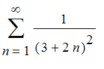
This series converges by comparison with the p-series . Each partial sum is bounded above by and the partial sums form an increasing sequence, so we know the sequence of partial sums converge. Checking to see what is programmed into Maple,

> sum(1/(3+2*n)^2,n=1..infinity)=
evalf(sum(1/(3+2*n)^2,n=1..infinity));

we get an exact sum. Check a few partial sums .

> seq(evalf(sum(1/(3+2*i)^2,i=1..100*n)),
n=1..5); n:='n':

>

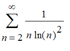
The function is a decreasing for n > 1 (Take the derivative), so we can use the integral test on this one.

> int(1/(n*(ln (n))^2),n=1..infinity);

Since the integral diverges, the series diverges.

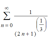This series diverges, since it is a p-series with p < 1

>

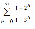
This series converges by comparison with .

> evalf(int(( n^5+4*n^3+1)/
(2*n^9+n^4+2 ),n=1..infinity));

>

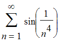This series converges by comparison with the 4-series.

> evalf(sum(sin(1/(n^4)),n=1..infinity));

>

Two interesting curves

The Snowflake Curve

The Snowflake Curve was initially described by Koch as an affirmative solution to the problem of whether there is a continuous curve that has no tangent line at any point on the curve.

It is defined as the limit of the sequence of curves generated by the procedure snowflake given below. Type in the words defined below and then enter snow(4) to get a feel for what the snowflake curve looks like. The first word performs a basic operation on any segment, which we think of as a list of its endpoints. It replaces the segment of length d with a sequence of four segments of length d/3 obtained in the following way: Start at the left endpoint of the segment and go d/3 of the way along the segment, turn left 60 degrees and go the same distance, turn right 60 degrees and go the same distance, then turn left 60 degrees and proceed d/3 units along the original segment to the right endpoint. Note that the resulting path has three points where there is no tangent.

> basic := proc(p1,p2)
local dx,dy, p3,p4,p5;
dx := (p2[1]-p1[1])/3.;
dy := (p2[2]-p1[2])/3.;
p3 := [p1[1]+dx,p1[2]+dy];
p4 := [p1[1]+2*dx,p1[2]+2*dy];
p5 := [p1[1]+1.5*dx-sqrt(3.)/2*dy,
p1[2]+1.5*dy+sqrt(3.)/2.*dx];
p3,p5,p4,p2;
end:

>

So for example, if we feed the points [0,0], [1,0] into basic, we get out the following sequence of numbers:

> basic([0,0],[1,0]);

>

Notice the left endpoint of the original segment is missing from this list. That is for programming reasons which become clear in the definition of the word flake below. The word flake takes a list of points, which represents a sequence of line segments laid end to end, and returns a list representing 4 times as many line segments, where each segment in the original list has been replaced by the 4 segments returned by basic.

>    flake := proc(fl)
    local i,curve;
        curve := fl[1];
        for i from 1 to nops(fl)-1 do
        curve :=   curve ,basic(fl[i],fl[i+1] ) ;
        od
    end:

Now the starting point for the snowflake curve is the equilateral triangle.

> curve := [[0,0],[1/2,1/2*sqrt(3)],[1,0],[0,0]];

To draw the second stage of the snowflake curve,

> plot([flake(curve)],scaling=constrained);

>

Now we can define the nth stage of the snowflake curve.

> snowflake := proc(n)
local i,curve,ti;
curve := [[0,0],[1/2,1/2*sqrt(3)],[1,0],[0,0]];
for i from 2 to n do curve := [flake(curve)] od;
ti := cat(n,`th stage of the snowflake curve`); plot(curve,color=black,style = LINE,
axes = NONE,scaling = CONSTRAINED,title = ti)
end:

> snowflake(4);

Here's an animation of the snowflake curve 'growing in place'. About 5 frames is all you can usefully see.

> plots[display]([seq(snowflake(i),i=1..5)],insequence=true,axes=none,scaling=constrained);

>

Problem: What is the length of the snowflake curve?

Solution: To calculate the length of the snowflake curve we see that the first stage has length units; the 2nd stage has length , or ; in general the nth stage has length , or 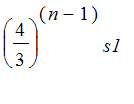. So the length of the nth stage goes to infinity as n gets large. This says the snowflake curve is infinitely long.

A Spacefiller

David Hilbert in 1891 described a continuous curve whose range is the unit square! This was contrary to the intuition of the time, which was that the range of a path had to be 1-dimensional. Here is a Maple word that draws an approximation to Hilbert's space filling curve . The approach to defining the drawing procedure peano (below) is similar to that used to define snowflake (above).

> basic := proc(p1,p2,p3)
local dx,dy,p4,p5,p6,p7,p8,p9;
p4 := .5*(p1+p2);
p9 := .5*(p2+p3);
p5 := p4+(p2-p9);
p6 := p2+(p2-p9);
p7 := p2+(p4-p1);
p8 := p9+(p4-p1);
p4,p5,p6, p2 ,p7,p8,p9, p3 ;
end:

>

> peano := proc(fl)
local i,cur;
cur := [fl[1] ] ;
for i from 1 by 2 to nops(fl)-2 do
cur := [op(cur),basic( fl[i],fl[i+1],fl[i+2] )]
od;

> end:

> fl := [[0,0],[1,1],[2,0]];

> for i from 1 to 4 do fl := peano(fl) od:
ti := cat(4,`th stage of Peano's curve`);
plot(fl,style=LINE,axes=NONE,title=ti,
scaling=CONSTRAINED);

>