Taylor's Theorem
Suppose the nth derivative of
![]() is defined at
is defined at
![]() . Then the nth
Taylor polynomial
for f at
. Then the nth
Taylor polynomial
for f at
![]() is defined as follows:
is defined as follows:
| > | p[n](x) = sum((D@@i)(f)(a)/i!*(x-a)^i,i=0..n); |
 = sum(`@@`(D,i)(f)(a)/i!*(x-a)^i,i = 0 .. n)](images/taylor4.gif)
The
Taylor remainder
function is defined as
![]()
There is a word, taylor , in the Maple vocabulary already which compute Taylor polynomials. Suppose we want the 11 th Taylor polynomial of the sin function at x = 0.
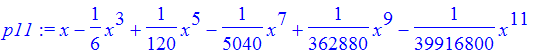
| > | p11 := taylor(sin(x),x=0,12); |

p11 is not actually a polynomial because of the term at the end which is used to signal which polynomial is represented (in case some of the coefficients are 0). We can convert to a polynomial.
| > | p11 := convert(p11,polynom); |
The Taylor polynomials are usually good approximations to the function near a. Let's plot the first few polynomials for the sin function at x =0.
| > | sinplot := plot(sin,-Pi..2*Pi,thickness=2): |
| > | tays:= plots[display](sinplot): for i from 1 by 2 to 11 do tpl := convert(taylor(sin(x), x=0,i),polynom): tays := tays,plots[display]([sinplot,plot(tpl,x=-Pi..2*Pi,y=-2..2, color=black,title=convert(tpl,string))]) od: |
| > | plots[display]([tays],view=[-Pi..2*Pi,-2..2]); |
![[Maple Plot]](images/taylor8.gif)
Just how close the polynomials are to the function is determined using Taylor's theorem below.
Theorem: (Taylor's remainder theorem) If the (n+1)st derivative of f is defined and bounded in absolute value by a number M in the interval from a to x, then
 <= M/(n+1)!*abs(x-a)^(n+1)](images/taylor9.gif)
This theorem is essential when you are using Taylor polynomials to approximate functions, because it gives a way of deciding which polynomial to use. Here's an example.
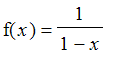
Problem Find the 2nd Taylor polynomial p[2] of
 at
at
![]() . Plot both the polynomial and f on the interval [.5,1.5]. Determine the maximum error in using p[2] to approximate ln(x) in this interval.
. Plot both the polynomial and f on the interval [.5,1.5]. Determine the maximum error in using p[2] to approximate ln(x) in this interval.
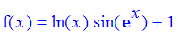
Solution:
| > | f := x -> ln(x)*sin(exp(x))+1; |
![]()
| > | fplot := plot(f,.5..1.5,thickness = 2): |
| > | p[2] := x -> sum((D@@i)(f)(1.)/i!*(x-1.)^i,i=0..2); |
![p[2] := proc (x) options operator, arrow; sum(`@@`(D,i)(f)(1.)/i!*(x-1.)^i,i = 0 .. 2) end proc](images/taylor13.gif)
| > | p[2](x); |
![]()
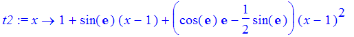
| > | t2 := unapply( convert(taylor(f(x),x=1,3),polynom),x); |
| > | tplot := plot(t2,1..1.5,color=black): |
| > | plots[display]([fplot,tplot]); |
![[Maple Plot]](images/taylor16.gif)
In order to use Taylor's remainder theorem, we need to find a bound M on the 3rd derivative of the function f. In this case, we could just plot the third derivative and eyeball an appropriate value for M.
| > | plot((D@@3)(f),.5..1.5) ; |
![[Maple Plot]](images/taylor17.gif)
We could use M = 75.
| > | M := 75; |
![]()
So the remainder
![]() is bounded by
is bounded by
| > | M/3!*(1.5-1)^3; |
![]()
| > |
We can see from the plot of f and the polynomial that the actual error is never more than about .1 on the interval [.5,1.5].
Another example :
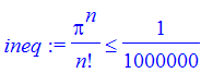
Which Taylor polynomial would you use to approximate the sin function on the interval from -Pi to Pi to within 1/10^6?
Solution:
Well, 1 is a bound on any derivative of the sin on any interval. So we need to solve the inequality
| > | ineq := 1/n!*Pi^n <= 1/10^6; |
for n. Solve will not be much help here because of the factorial, but we can find the smallest n by running through a loop.
| > | n := 1: while evalf(1/n!*Pi^n) > 1/10^6 do n := n+1 od: print (`take n to be `,n); |
![]()
| > | (seq(evalf( 1/n!*Pi^n) ,n=15..20)); |
![]()
| > | restart; |
| > | t17 := convert(taylor(sin(x),x=0,18),polynom); |
![]()

| > | plot(t17,x=-Pi..Pi); |
![[Maple Plot]](images/taylor26.gif)
Looks pretty much like the sin function.
Problems
Exercise: Show that
![]() is approximated to within 7 decimals by
is approximated to within 7 decimals by
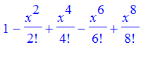 for all x in
![[-Pi/4, Pi/4]](images/taylor29.gif) .
.
Exercise: Use taylor and convert(..,polynom) to compute and plot, on the interval specified, the first few taylor polynomials of the following functions. Observe the convergence of the polynomials to the function and make comments.
![]() at x=1, on the interval [-1,3].
at x=1, on the interval [-1,3].
 at x =0 on the interval [-2,2]
![]() at x = 0 on the interval [-2..2]
at x = 0 on the interval [-2..2]
Exercise: Write a procedure to compute sin(x) for any x by using p[5]. restricted to the interval [0,Pi/4].
Outline of solution
: If x is negative, replace x with
![]() and use the oddness
and use the oddness
![]() property. If x is greater than or equal to 2*Pi, then replace x with x-2*Pi and use the periodicity
property. If x is greater than or equal to 2*Pi, then replace x with x-2*Pi and use the periodicity
![]() . Repeat this step until [0, 2*Pi ). If Pi/4 < x < Pi/2 , then use the trig indentity
. Repeat this step until [0, 2*Pi ). If Pi/4 < x < Pi/2 , then use the trig indentity
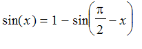
and approximate
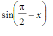 by
by
](images/taylor38.gif) . If
. If
 and
and
![]() , then
, then
![]() . If
. If
![]() and
and
![]() , then
, then
![]() .
.
| > |
| > |
Exercise: Find the smallest n such that the nth Taylor polynomial p[n](x) for
 at
at
![]() approximates exp(x) to within
approximates exp(x) to within
 for x in [0,1]. (You will want to set
Digits
equal to 15 in order to do this one.
for x in [0,1]. (You will want to set
Digits
equal to 15 in order to do this one.
| > |
or so to do this problem.)
| > |
| > |