> with(DEtools); -1


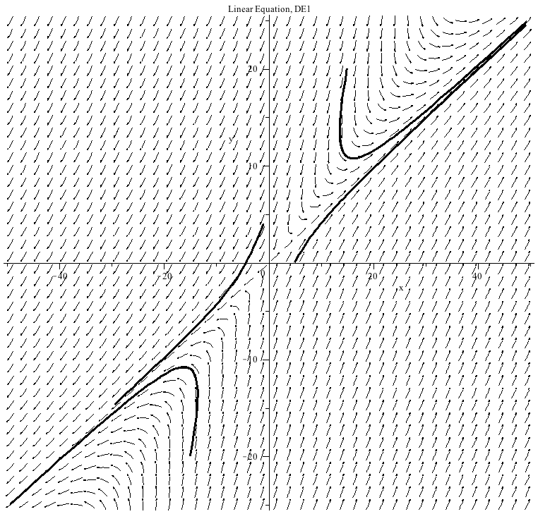
This system of differential equations (DE1) has two eigenvalues of opposite sign (λ=1 and λ=−2). The point (0,0) is unstable and called a saddle point. 

> `assign`(DE1, diff(x(t), t) = `+`(`*`(2, `*`(x(t))), `-`(`*`(2, `*`(y(t))))), diff(y(t), t) = `+`(`*`(2, `*`(x(t))), `-`(`*`(3, `*`(y(t)))))); 1
`assign`(DE1, diff(x(t), t) = `+`(`*`(2, `*`(x(t))), `-`(`*`(2, `*`(y(t))))), diff(y(t), t) = `+`(`*`(2, `*`(x(t))), `-`(`*`(3, `*`(y(t)))))); 1
 

diff(x(t), t) = `+`(`*`(2, `*`(x(t))), `-`(`*`(2, `*`(y(t))))), diff(y(t), t) = `+`(`*`(2, `*`(x(t))), `-`(`*`(3, `*`(y(t))))) (1)
 

> DEplot({DE1}, [x(t), y(t)], t = 0 .. 2, [[x(0) = -1, y(0) = 4], [x(0) = 5, y(0) = 0], [x(0) = 15, y(0) = 20], [x(0) = -15, y(0) = -20]], numsteps = 76, title =
DEplot({DE1}, [x(t), y(t)], t = 0 .. 2, [[x(0) = -1, y(0) = 4], [x(0) = 5, y(0) = 0], [x(0) = 15, y(0) = 20], [x(0) = -15, y(0) = -20]], numsteps = 76, title =
 

Plot_2d
 

> `assign`(DE2, diff(x(t), t) = `+`(`*`(2, `*`(x(t))), `-`(`*`(3, `*`(y(t))))), diff(y(t), t) = `+`(x(t), `-`(`*`(2, `*`(y(t)))))); 1
`assign`(DE2, diff(x(t), t) = `+`(`*`(2, `*`(x(t))), `-`(`*`(3, `*`(y(t))))), diff(y(t), t) = `+`(x(t), `-`(`*`(2, `*`(y(t)))))); 1
 

diff(x(t), t) = `+`(`*`(2, `*`(x(t))), `-`(`*`(3, `*`(y(t))))), diff(y(t), t) = `+`(x(t), `-`(`*`(2, `*`(y(t))))) (2)
 

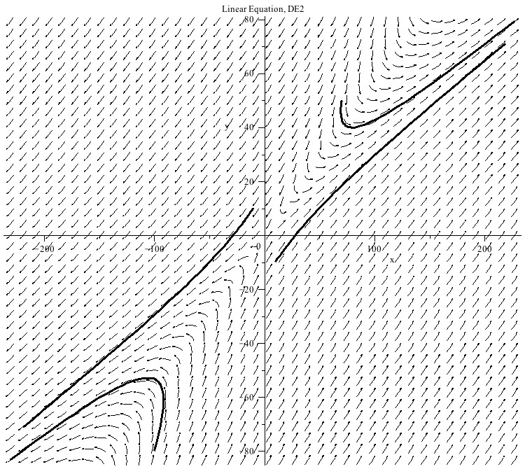
This system of differential equations (DE2) has two eigenvalues of opposite sign (λ=1 and λ=−1). The point (0,0) is unstable and called a saddle point. 

> DEplot({DE2}, [x(t), y(t)], t = 0 .. 2, [[x(0) = 10, y(0) = -10], [x(0) = 70, y(0) = 50], [x(0) = -10, y(0) = 10], [x(0) = -100, y(0) = -80]], numsteps = 76, title =
DEplot({DE2}, [x(t), y(t)], t = 0 .. 2, [[x(0) = 10, y(0) = -10], [x(0) = 70, y(0) = 50], [x(0) = -10, y(0) = 10], [x(0) = -100, y(0) = -80]], numsteps = 76, title =
 

Plot_2d
 

> `assign`(DE3, diff(x(t), t) = `+`(`-`(`*`(3, `*`(x(t)))), `*`(sqrt(2), `*`(y(t)))), diff(y(t), t) = `+`(`*`(sqrt(2), `*`(x(t))), `-`(`*`(2, `*`(y(t)))))); 1
`assign`(DE3, diff(x(t), t) = `+`(`-`(`*`(3, `*`(x(t)))), `*`(sqrt(2), `*`(y(t)))), diff(y(t), t) = `+`(`*`(sqrt(2), `*`(x(t))), `-`(`*`(2, `*`(y(t)))))); 1
 

diff(x(t), t) = `+`(`-`(`*`(3, `*`(x(t)))), `*`(`^`(2, `/`(1, 2)), `*`(y(t)))), diff(y(t), t) = `+`(`*`(`^`(2, `/`(1, 2)), `*`(x(t))), `-`(`*`(2, `*`(y(t))))) (3)
 

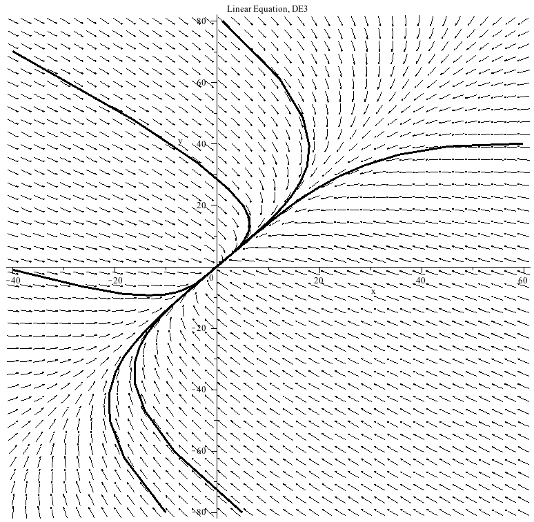
This system of differential equations (DE3) has two negative eigenvalues (λ=−1 and λ=−4). The point (0,0) is called a sink or a stable node. 

> DEplot({DE3}, [x(t), y(t)], t = 0 .. 7, [[x(0) = -40, y(0) = 70], [x(0) = -10, y(0) = -80], [x(0) = 60, y(0) = 40], [x(0) = 1, y(0) = 80], [x(0) = -40, y(0) = -1], [x(0) = 5, y(0) = -80]], numsteps = ...
DEplot({DE3}, [x(t), y(t)], t = 0 .. 7, [[x(0) = -40, y(0) = 70], [x(0) = -10, y(0) = -80], [x(0) = 60, y(0) = 40], [x(0) = 1, y(0) = 80], [x(0) = -40, y(0) = -1], [x(0) = 5, y(0) = -80]], numsteps = ...
 

Plot_2d
 

> `assign`(DE4, diff(x(t), t) = `+`(`*`(3, `*`(x(t))), `*`(2, `*`(y(t)))), diff(y(t), t) = `+`(x(t), `*`(2, `*`(y(t))))); 1
`assign`(DE4, diff(x(t), t) = `+`(`*`(3, `*`(x(t))), `*`(2, `*`(y(t)))), diff(y(t), t) = `+`(x(t), `*`(2, `*`(y(t))))); 1
 

diff(x(t), t) = `+`(`*`(3, `*`(x(t))), `*`(2, `*`(y(t)))), diff(y(t), t) = `+`(x(t), `*`(2, `*`(y(t)))) (4)
 

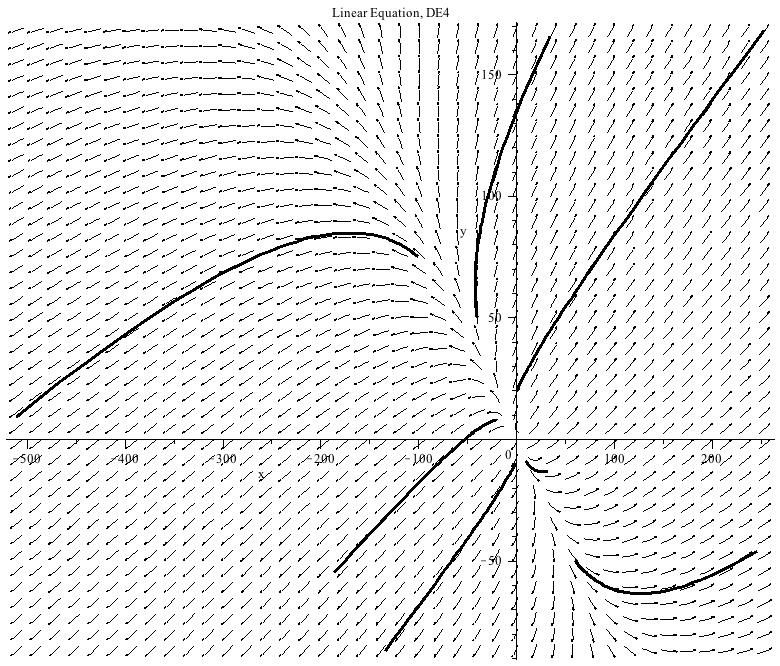
This system of differential equations (DE4) has two positive eigenvalues (λ=1 and λ=4). The point (0,0) is called a source or an unstable node. 


> DEplot({DE4}, [x(t), y(t)], t = 0 .. .75, [[x(0) = -40, y(0) = 50], [x(0) = 1, y(0) = 20], [x(0) = -1, y(0) = -10], [x(0) = -20, y(0) = 8], [x(0) = 60, y(0) = -50], [x(0) = -100, y(0) = 75], [x(0) = 1...
DEplot({DE4}, [x(t), y(t)], t = 0 .. .75, [[x(0) = -40, y(0) = 50], [x(0) = 1, y(0) = 20], [x(0) = -1, y(0) = -10], [x(0) = -20, y(0) = 8], [x(0) = 60, y(0) = -50], [x(0) = -100, y(0) = 75], [x(0) = 1...
 

Plot_2d
 

> `assign`(DE5, diff(x(t), t) = `+`(`-`(x(t)), `-`(y(t))), diff(y(t), t) = x(t)); 1
 

diff(x(t), t) = `+`(`-`(x(t)), `-`(y(t))), diff(y(t), t) = x(t) (5)
 

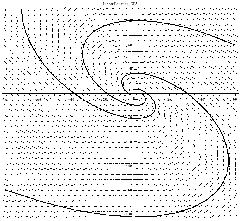
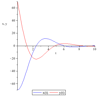
This system of differential equations (DE5) has two complex conjugate eigenvalues (λ=-`/`(1, 2) ±`+`(`*`(`/`(1, 2), `*`(i)))sqrt(3)) with a negative real part. The point (0,0) is called a stable spiral. 

> DEplot({DE5}, [x(t), y(t)], t = 0 .. 7, [[x(0) = -70, y(0) = 70], [x(0) = -80, y(0) = -80], [x(0) = 60, y(0) = 40]], numsteps = 76, title =
DEplot({DE5}, [x(t), y(t)], t = 0 .. 7, [[x(0) = -70, y(0) = 70], [x(0) = -80, y(0) = -80], [x(0) = 60, y(0) = 40]], numsteps = 76, title =
 

Plot_2d
 

> with(plots); -1
 

> `assign`(fcns, {x(t), y(t)}); 1
 

{x(t), y(t)} (6)
 

> `assign`(sol5, dsolve({DE5, x(0) = -70, y(0) = 70}, fcns, type = numeric, method = classical)); 1
`assign`(sol5, dsolve({DE5, x(0) = -70, y(0) = 70}, fcns, type = numeric, method = classical)); 1
 

proc (x_classical) local _res, _dat, _vars, _solnproc, _xout, _ndsol, _pars, _n, _i; option `Copyright (c) 2000 by Waterloo Maple Inc. All rights reserved.`; if `<`(1, nargs) then error (7)
 

> odeplot(sol5, [[t, x(t)], [t, y(t)]], 0 .. 10, color = [
odeplot(sol5, [[t, x(t)], [t, y(t)]], 0 .. 10, color = [
 

Plot_2d
 

> `assign`(DE6, diff(x(t), t) = `+`(x(t), `-`(y(t))), diff(y(t), t) = x(t)); 1
 

diff(x(t), t) = `+`(x(t), `-`(y(t))), diff(y(t), t) = x(t) (8)
 

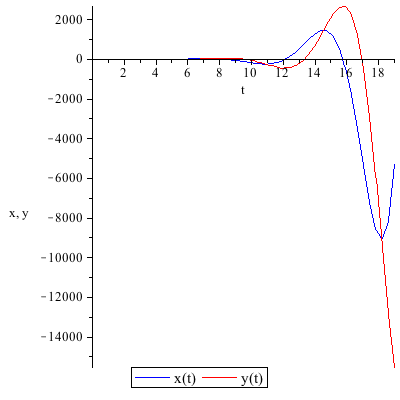
This system of differential equations (DE6) has two complex conjugate eigenvalues (λ=`/`(1, 2) ±`+`(`*`(`/`(1, 2), `*`(i)))sqrt(3)) with a positive real part. The point (0,0) is called an unstable spiral. 
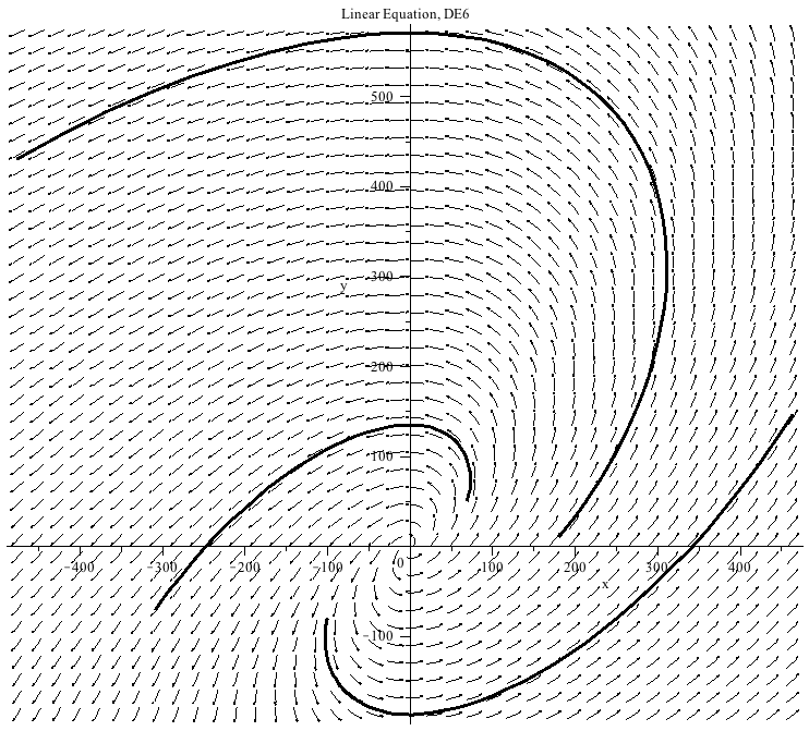
> DEplot({DE6}, [x(t), y(t)], t = 0 .. 3, [[x(0) = 70, y(0) = 50], [x(0) = -100, y(0) = -80], [x(0) = 180, y(0) = 10]], numsteps = 76, title =
DEplot({DE6}, [x(t), y(t)], t = 0 .. 3, [[x(0) = 70, y(0) = 50], [x(0) = -100, y(0) = -80], [x(0) = 180, y(0) = 10]], numsteps = 76, title =
 

Plot_2d
 

> with(plots); -1
 

> `assign`(fcns6, {x(t), y(t)}); 1
 

{x(t), y(t)} (9)
 

> `assign`(sol6, dsolve({DE6, x(0) = 1, y(0) = 1}, fcns6, type = numeric, method = classical)); 1
`assign`(sol6, dsolve({DE6, x(0) = 1, y(0) = 1}, fcns6, type = numeric, method = classical)); 1
 

proc (x_classical) local _res, _dat, _vars, _solnproc, _xout, _ndsol, _pars, _n, _i; option `Copyright (c) 2000 by Waterloo Maple Inc. All rights reserved.`; if `<`(1, nargs) then error (10)
 

> odeplot(sol6, [[t, x(t)], [t, y(t)]], 0 .. 19, color = [
odeplot(sol6, [[t, x(t)], [t, y(t)]], 0 .. 19, color = [
 

Plot_2d
 

>