|
|
College Algebra |
Chapter 3: Polynomial Equations
3.1 Polynomials
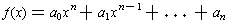
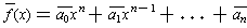
A polynomial p(x) with coefficients in a field F is an expression
of the form
 where the
coefficients
where the
coefficients
 are in F, and n is a non-negative integer. Each of
the summands is called a term of the polynomial. If
are in F, and n is a non-negative integer. Each of
the summands is called a term of the polynomial. If
 , then n is called the degree of the polynomial. The
degree of the zero polynomial is defined to be -1. If
, then n is called the degree of the polynomial. The
degree of the zero polynomial is defined to be -1. If
 , then
the coefficient
, then
the coefficient
 is called the leading coefficient of the
polynomial p(x). If the leading coefficient of the p(x) is 1, the
polynomial is said to be monic. The set of all polynomials with
coefficients in F is denoted F[x].
is called the leading coefficient of the
polynomial p(x). If the leading coefficient of the p(x) is 1, the
polynomial is said to be monic. The set of all polynomials with
coefficients in F is denoted F[x].
A rational function of one variable
is a fraction p(x)/q(x) where p and q are polynomials with coefficients in F
and
 . (Note: we mean rational functions to simply be an
expression of this form; we are not thinking of it as being an actual
function.) The set of all rational functions of one variable x is denoted
F(x).
. (Note: we mean rational functions to simply be an
expression of this form; we are not thinking of it as being an actual
function.) The set of all rational functions of one variable x is denoted
F(x).
We can define operations on polynomials in the usual manner. The
sum of two polynomials is obtained by taking the sums of the coefficients.
If
 and
and
 are two
polynomials, then their product is obtained by taking the sum of all the
terms of the form
are two
polynomials, then their product is obtained by taking the sum of all the
terms of the form
 and collecting the terms with the
same powers of x. This is precisely what one would do if you just expanded
the product using the distributive law. One can extend in the obvious
way, these operations to operations on rational functions.
and collecting the terms with the
same powers of x. This is precisely what one would do if you just expanded
the product using the distributive law. One can extend in the obvious
way, these operations to operations on rational functions.
Although tedious, it is straightforward to show that the rational functions of one variable with coefficients in a field F form a field.
Example 1: Let F is an ordered field. A rational function f(x) of one variable with coefficients in F can be expressed as f(x) = cp(x)/q(x) where p(x) and q(x) are monic and c is in F. We say that such a rational function is positive if and only if c is positive. One can show that this makes the field of rational functions of one variable with coefficients in F into an ordered field. It is an example of an ordered field which is NOT Archimedean.
Recall from high school algebra that one can do long division of polynomials to obtain a polynomial quotient and a polynomial remainder whose degree is smaller than that of the divisor. In summary:
Proposition 1: (Division Theorem) If p(x) and d(x) are polynomials
with coefficients in a field F and
 , then there are unique
polynomials q(x) and r(x) with coefficients in F such that p(x) = q(x)d(x) + r(x)
and the degree of r(x) is less than the degree of d.
, then there are unique
polynomials q(x) and r(x) with coefficients in F such that p(x) = q(x)d(x) + r(x)
and the degree of r(x) is less than the degree of d.
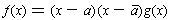
Corollary 1: If f(x) is a polynomial with coefficients in a field F and a in F is a root of f(x) = 0, the f(x) = (x - a)q(x) for some polynomial q(x) with coefficients in F.
Proof: By Proposition 1, we have f(x) = (x - a)q(x) + r(x) where r(x) has degree less than 1. But then r(x) is a constant. Furthermore, 0 = f(a) = (a - a)q(a) + r(a) = r(a). So r(a) = 0. Since r is a constant, this means that r = 0.
Corollary 2: If f(x) is a non-zero polynomial of degree n with coefficients in a field F, then f has at most n roots in f.
Proof: If it is false, we can can choose an f of smallest degree for which it is false. If a is a root, then f(x) = (x - a)q(x) where q is of degree n - 1. If f has more than n roots including x = a, then this equation shows that q has at least n roots other than x = a. This contradicts the choice of f as being a counterexample of smallest degree.
In particular, any element of F has at most n
 -roots. So, the
list of roots we found by Corollary 8 in section 2.8.2 is complete.
-roots. So, the
list of roots we found by Corollary 8 in section 2.8.2 is complete.
Let f(x) and g(x) be two polynomials with coefficients in a field F. Then f(x) is a divisor of g(x) if and only if there is a polynomial q(x) with coefficients in F such that g(x) = f(x)q(x). Note that the degrees are related by

One says that f(x) is a proper divisor of g(x) if f(x) is a divisor of g(x), f(x) is not a constant, and f(x) has degree less than that of g(x). The polynomial f(x) is said to be irreducible if it is non-zero and has no proper divisors.
Basically, irreducible polynomials play the same role as did prime numbers. Just as with the natural numbers, the division theorem can be used to define the Euclidean Algorithm which allows one to calculate the greatest common divisor of two polynomials and to express it as a linear combination of the two original polynomials. The only difference here is that we compare polynomials using their degrees; so, for example, the greatest common divisor is any common divisor with largest possible degree. Details are given in the exercises.
One has:
Proposition 2: (Unique Factorization) Every non-zero polynomial over a field F can be factored into a product of zero or more irreducible polynomials. If f(x) is a non-zero monic polynomial, then every non-zero polynomial factors uniquely (up to order) into a product of monic irreducible polynomials.
Proof: This proof is also completely parallel to the one with natural numbers and so is left to the exercises.
3.2.1 Graphing near a Point
Let's start off by assuming that our polynomials f(x) have real number coefficients and that we are evaluating them for real values of the variable x.
Behavior near zero. How can you approximate the graph of a
polynomial function
 for
values of x near 0? The idea is that x being near zero means that
for
values of x near 0? The idea is that x being near zero means that
 is
small. But then
is
small. But then
 is much smaller than zero -- for example, if
 ,
then
,
then
 , which says that the absolute value of the square is
a hundredth the size of the absolute value of x. For higher powers, the
numbers are even smaller; for example,
, which says that the absolute value of the square is
a hundredth the size of the absolute value of x. For higher powers, the
numbers are even smaller; for example,
 is at most one ten thousandth
the size of the absolute value of x. In terms of what you can see in the graph,
this means that only the low degree terms have visible effects.
is at most one ten thousandth
the size of the absolute value of x. In terms of what you can see in the graph,
this means that only the low degree terms have visible effects.
- For x near zero, the graph of y = f(x) is close to the graph of the constant function y = f(0).
- If you take the constant term and the term of lowest positive degree,
then, for x close to zero, the graph of y = f(x) is approximately the
same as the graph of this much simpler function.
- For example if the coefficient of x is non-zero, then our new function
looks like
 . This is a straight line with slope
equal to the coefficient of the x term. (To see this, graph any
polynomial function on your calculator -- regardless of how curved the
graph looks, it straightens out as soon as you zoom in on the value at zero.)
. This is a straight line with slope
equal to the coefficient of the x term. (To see this, graph any
polynomial function on your calculator -- regardless of how curved the
graph looks, it straightens out as soon as you zoom in on the value at zero.)
- If the coefficient of x is zero, but the coefficient of
 is
non-zero, then our new function looks like
is
non-zero, then our new function looks like
 . This
is a parabola. If
. This
is a parabola. If
 , the parabola opens upward and the graph
takes on its smallest value
, the parabola opens upward and the graph
takes on its smallest value
 at x = 0. Our original function does
the same for x sufficiently close to zero; we say that the function has
a local minimum at x = 0. If
at x = 0. Our original function does
the same for x sufficiently close to zero; we say that the function has
a local minimum at x = 0. If
 , the parabola opens
downward, and so the function is biggest at x = 0; one says that the
function has a local maximum at x = 0.
, the parabola opens
downward, and so the function is biggest at x = 0; one says that the
function has a local maximum at x = 0.
- For example if the coefficient of x is non-zero, then our new function
looks like
Examples: The function
 can be approximated
for x near zero by
can be approximated
for x near zero by
 ; the graph of f looks like a straight
line with slope -3 near 0. (Of course, this is only true very close to zero.)
; the graph of f looks like a straight
line with slope -3 near 0. (Of course, this is only true very close to zero.)
The function
 is approximated by
 for x close to zero.
 has a local maximum at x = 0.
Behavior near x = a We want to see how a
polynomial function
 behaves
near a fixed value x = a. The previous discussion told us how to do this
when a = 0. When a is not zero, we can simply apply our previous discussion
to the polynomial g(x) = f(a + x).
behaves
near a fixed value x = a. The previous discussion told us how to do this
when a = 0. When a is not zero, we can simply apply our previous discussion
to the polynomial g(x) = f(a + x).
Examples: Let
 . We have seen that near x = 0,
the graph is approximated by the straight line y = -3x + 4. Suppose
we wanted to know what it looked like near x = 2? Let
. We have seen that near x = 0,
the graph is approximated by the straight line y = -3x + 4. Suppose
we wanted to know what it looked like near x = 2? Let
 .
One has
.
One has

So, the graph of y = f(x) near x = 2 is the same as the graph of y = g(x) near zero, and it is approximated by y = 9x + 6. So, the graph of y = f(x) near x = 2 looks like a straight line with slope 9 and passing through (2, 6).
If we are interested in what the graph of y = f(x) looks like near x = -1, then consider g(x) = f(-1 + x):

So, the graph of y = f(x) near x = -1 is the same as the graph of y = g(x)
near x = 0, which is approximated by
 . So, the graph of
y = f(x) has a local maximum at x = -1.
. So, the graph of
y = f(x) has a local maximum at x = -1.
As a final example, check you understanding by showing that the function f(x) has a local minimum at x = 1.
Derivatives. As the example shows, it can be quite tiresome to
keep computing g(x) = f(a + x) for various values of a. So, what is a
short-cut? Note that
 for every k.
By substituting, it is easy to see that
for every k.
By substituting, it is easy to see that

where

The polynomial f'(y) is called the derivative of f(x). We have just seen that the graph of y = f(x) is approximated near x = a by a straight line with slope f'(a) through the point (a, f(a)).
Large values of x. When x is large in absolute value, the
polynomial function
 behaves
like its term of highest degree. This is because
behaves
like its term of highest degree. This is because
 is much bigger
than
is much bigger
than
 and all the other terms. In particular, if
 , then
for x positive and large in absolute value, f(x) is positive and very large
in absolute value. If
, then
for x positive and large in absolute value, f(x) is positive and very large
in absolute value. If
 , then f(x) is negative and large in
absolute value when x is positive and large in absolute value.
, then f(x) is negative and large in
absolute value when x is positive and large in absolute value.
When x is negative and large in absolute value,
 will be large
in absolute value, but its sign will be either negative or positive depending
on whether n is odd or even.
will be large
in absolute value, but its sign will be either negative or positive depending
on whether n is odd or even.
Complex polynomials. If the
polynomial function
 has
complex coefficients and we allow x to range through complex values, then
we can still get an idea of how the function behaves near particular points.
has
complex coefficients and we allow x to range through complex values, then
we can still get an idea of how the function behaves near particular points.
- For x near 0, the function y = f(x) behaves like its low degree terms.
(If |x| is small, then
 is smaller still, etc.) So, y = f(x)
is approximated by
is smaller still, etc.) So, y = f(x)
is approximated by
 or more generally by the sum of
the constant term and term of lowest positive degree.
or more generally by the sum of
the constant term and term of lowest positive degree.
- For x near the complex number a, the function y = f(x) behaves like g(x) = f(a + x) near x = 0.
- When x is large in absolute value, then f(x) is dominated by its
highest degree term, and so f(x) is approximated by
 . In particular,
if f is not a constant, then |f(x)| is large as soon as |x| is.
. In particular,
if f is not a constant, then |f(x)| is large as soon as |x| is.
In the case of real polynomials, |f(x)| be smallest at x = a for
all x near a even though
 . For example,
 has a local minimum at x = 0 and
 .
.
This only happens because we restrict the values of x to be real.
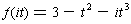
For example, if we allowed x = it, then
 takes on
values f(it) smaller than 3 for all sufficiently small real values of t.
takes on
values f(it) smaller than 3 for all sufficiently small real values of t.
One can do the same thing for a general polynomial.
If we approximate f(x) by its constant term and its
term of lowest positive degree, then
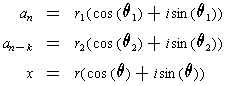
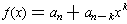 . Then
we can write the numbers in polar form:
. Then
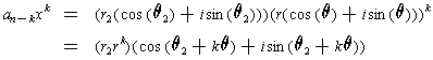
we can write the numbers in polar form:
Then one has
Now, if
 is non-zero, we can choose
 so that the angle of
this last equation differs from
so that the angle of
this last equation differs from
 by precisely
 . If we did
this, then the sum of the two terms would be smaller in absolute value
than
. If we did
this, then the sum of the two terms would be smaller in absolute value
than
 provided that r is not too large. What one has shown is:
Lemma (d'Alembert): If f(x) is a non-constant polynomial with complex
coefficients and
 for some complex value
 , then there are
complex numbers x arbitrarily close to
, then there are
complex numbers x arbitrarily close to
 for which
 .
.
3.2 Rational Roots
If f(x) = 0 is a non-zero polynomial equation with integer coefficients, then there are at most a finite number of possible rational number roots:
Proposition 3: Consider the equation

where the coefficients are integers and
 and
and
 . Any
rational root of this equation must be expressible in the form
. Any
rational root of this equation must be expressible in the form
 where
p is a divisor of
where
p is a divisor of
 and q is a divisor of
 .
.
Proof: Suppose x = a/b is a root of the equation where a and b are integers with a and b are relatively prime. Both a and b are non-zero. Substituting x = a/b into the equation, one gets

Multiplying through by
 gives
gives

The first n terms are all multiples of a and so a divides
 . On the
other hand, b is a divisor of the last n terms; so b divides
. On the
other hand, b is a divisor of the last n terms; so b divides
 .
The result now follows from these two assertions and
.
The result now follows from these two assertions and
Lemma 1: Let a, b, and c be integers with
 . If a and b
are relatively prime and a divides the product cb,
then a divides c.
. If a and b
are relatively prime and a divides the product cb,
then a divides c.
Proof: If the result were false, then there would be a counter-example
with a having smallest possible absolute value. One has ae = cb for some integer
e. Clearly a is not 1. Let a
= pq where p is a prime and q an integer. Then p also divides cb and p is
relatively prime to b. By Corollary 3 of Section 2.6, it follows that p
divides c, say c = pr with r an integer. since ae = cb, we have
pqe = prb and so p(qe - rb) = 0. Since
 , it follows that qe = rb
and q is a proper divisor of a. In particular, q is also relatively prime to b.
This contradicts the minimality of the choice of a, and proves the lemma.
, it follows that qe = rb
and q is a proper divisor of a. In particular, q is also relatively prime to b.
This contradicts the minimality of the choice of a, and proves the lemma.
Example 2: i. The square root of 2 is irrational because it is
a root of
 and is different from -2, -1, 1, and 2.
ii. The equation f(x) = 1 has no rational solutions where
 because both f(1) and f(-1) are non-zero.
iii. Consider the quartic equation
 . The possible
roots are 10, 10/2 = 5, 10/3, 10/6, 5, 5/2, 5/3, 5/6, 2, 2/2 = 1, 2/3, 2/6 = 1/3,
1, 1/2, 1/3, 1/6 and the negatives of these numbers. Substituting these
into the equation, one eventually discovers that the first of these that
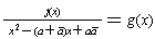
is a root is x = 5/2. Since it is a root, we can apply the division theorem;
x - 5/2 is a divisor of the quartic. Dividing out we are reduced to a cubic
equation:
. The possible
roots are 10, 10/2 = 5, 10/3, 10/6, 5, 5/2, 5/3, 5/6, 2, 2/2 = 1, 2/3, 2/6 = 1/3,
1, 1/2, 1/3, 1/6 and the negatives of these numbers. Substituting these
into the equation, one eventually discovers that the first of these that
is a root is x = 5/2. Since it is a root, we can apply the division theorem;
x - 5/2 is a divisor of the quartic. Dividing out we are reduced to a cubic
equation:
 . Dividing out by 2, we get
 The possible rational roots of the new
equation are: 2/1 = 2, 2/3, 1/1 = 1, and 1/3 as well as the negatives of
all these numbers. Checking each of the possibilities, we see that x = 2/3
is a root. Again, we can divide by x - 2/3 to get
The possible rational roots of the new
equation are: 2/1 = 2, 2/3, 1/1 = 1, and 1/3 as well as the negatives of
all these numbers. Checking each of the possibilities, we see that x = 2/3
is a root. Again, we can divide by x - 2/3 to get
 This is a quadratic; so we know we can solve it completely. In our case
the two roots are
This is a quadratic; so we know we can solve it completely. In our case
the two roots are
 . So the original equation has rational
roots 5/2 and 2/3 as well as two complex roots
. So the original equation has rational
roots 5/2 and 2/3 as well as two complex roots
 .
.
Remark 1: An examination of the proof of the Proposition should
convince you that it basically only depended on the unique factorization of integers.
In the last section, we saw that for any field F, the polynomials with
coefficients in F also factor uniquely. In particular, the same argument
therefore tells us about the rational function solutions of polynomial
equations with coefficients in F[y]. This would show, for example, that there is NO rational
function which is a square root of
 .
.
3.3 The Fundamental Theorem of Algebra
We will not be ready to prove this result until we get to Chapter 5, but we can at least state the result and see a few of its consequences.
Theorem 1: (Fundamental Theorem of Algebra) Every non-constant polynomial f(x) with complex number coefficients has at least one complex number root.
Corollary 2: Every non-zero polynomial f(x) with complex number coefficients can be factored into a product of linear polynomials with complex coefficients.
Proof: This is a simple descent argument using the Fundamental Theorem of Algebra and the Division Theorem.
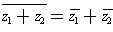
The complex conjugate
 of the complex number z = a + bi is
defined by
of the complex number z = a + bi is
defined by
 . Geometrically, this is reflection across
the x-axis in the complex plane.
. Geometrically, this is reflection across
the x-axis in the complex plane.
Proposition 4: The complex conjugate function
 satisfies
-
-

- If r is a real number, then
 . Conversely, if
 ,
then z is a real number.
,
then z is a real number.
- The complex conjugate of the complex conjugate of any complex number is equal to the original complex number.
Proof: Let us prove the second assertion leaving the other two
as exercises. Let
 for j = 1, 2. Then expanding the
left side gives:
for j = 1, 2. Then expanding the
left side gives:
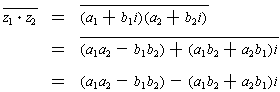
Expanding the right side gives
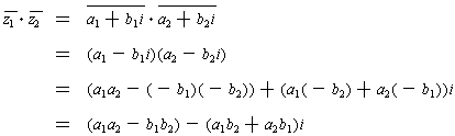
which is the same as the expansion of the left side.
Corollary 3: For any complex number z and natural number n, one
has
 .
.
Proof: This follows by induction (or descent).
Given a polynomial
 with
complex coefficients, one
can define the conjugate of f by applying the complex conjugate function to
each of the coefficients, i.e.
with
complex coefficients, one
can define the conjugate of f by applying the complex conjugate function to
each of the coefficients, i.e.
 .
.
Corollary 4: If f(x) is a polynomial with complex coefficients
and z is a complex number, then
 .
.
Proof: This is another descent argument.
Corollary 5: If f(x) = 0 where f is a non-zero polynomial with
real coefficients has a complex root z, then
 is also a root
of the same equation.
is also a root
of the same equation.
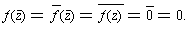
Proof: Since f has real coefficients,
 .
So,
.
So,
Corollary 6: If f(x) is a non-zero polynomial with real coefficients,
then the non-real complex roots of f(x) = 0 occur in complex conjugate
pairs (i.e. If z is a root, so is
 .). In particular, the
polynomial f(x) factors into a product of zero or more linear and quadratic polynomials
with real coefficients.
.). In particular, the
polynomial f(x) factors into a product of zero or more linear and quadratic polynomials
with real coefficients.
Proof: The first assertion is just Corollary 5. If the second assertion were false, then choose a counter-example f of minimal degree. Clearly f is not a constant; so it has at least one complex root. If f has a real root a, then the Division Theorem says that f(x) = (x - a) g(x) where g is a polynomial with real coefficients. Since g has lower degree than f, the assertion is true for g, but then substituting shows that it is also true of f, which would be contradiction.
So, f must have no real roots. Suppose f has a non-real complex root a.
Then Corollary 5 tells us that
 is also a root of f. Applying the
Division Theorem twice, we get
is also a root of f. Applying the
Division Theorem twice, we get
 where g
has complex coefficients. Now,
where g
has complex coefficients. Now,
 Now, the coefficients of this quadratic are equal to their complex conjugate; so
the last proposition says that the quadratic has real coefficients. Since
f also has real coefficients,
Now, the coefficients of this quadratic are equal to their complex conjugate; so
the last proposition says that the quadratic has real coefficients. Since
f also has real coefficients,
 also has real coefficients. But g has degree less than the degree of f; so
it is a product of zero or more linear and quadratic polynomials with
real coefficients. But then so is f(x), which again is a contradiction.
also has real coefficients. But g has degree less than the degree of f; so
it is a product of zero or more linear and quadratic polynomials with
real coefficients. But then so is f(x), which again is a contradiction.
Corollary 6: Every non-zero polynomial of odd degree with real coefficients has at least one real root.
Proof: Since the non-real roots occur in complex conjugate pairs, the only way for there to be no real roots would be if the degree were even.
3.4 Cubic Equations
Whereas the solution of quadratic equations was known in some form from the time of the Babylonians, the solution of the general cubic equation was first discovered perhaps by Tartaglia and published by Cardan during the Renaissance. It represented a giant leap forward; the most spectacular achievement showing for the first time in close to two millenia that the great achievement of the classical civilizations could be bettered.
The problem is to find solutions of the general cubic
equation
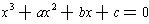 where a, b, and c are complex numbers.
Reduction Step: To understand the first step, recall how we solved quadratic equations.
The idea was that they were easy to solve if the linear term was missing.
So, the idea was to make the middle term disappear. Starting with
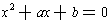 , one could write this as
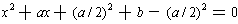 .
The additional term was chosen so that one would get a perfect square, i.e.
so that we could factor it to get
.
The additional term was chosen so that one would get a perfect square, i.e.
so that we could factor it to get
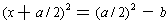 . This is
just like one of the quadratics without a linear term and so is easy to solve.
. This is
just like one of the quadratics without a linear term and so is easy to solve.
In the case of a cubic, we can attempt the same trick. And it does help somewhat. In this case we have a cubic and so, if we cube (x + d) we would get
. Comparing this with our cubic, we see that we can make the quadratic term match by taking d = a/3. This gives:

This looks very complicated, but the idea is that, if we think of x + a/3 as being a new variable, say y, then the polynomial is a cubic in y without any quadratic term. We have shown:
Lemma 2: By making a linear substitution x = y - a/3, the general cubic can be written as a cubic with no quadratic term. So, to solve the general cubic, it is enough to handle the case where the quadratic term is zero.
The above reduction step was well known at the time and does not
represent any great achievement. To understand the next step, again consider
the case of quadratics. If
 has roots
 and
and
 ,
then the Division Theorem tells us that
,
then the Division Theorem tells us that
 . Multiplying
this out, we get
. Multiplying
this out, we get
 Comparing these with
our original coefficients, we see that
Comparing these with
our original coefficients, we see that
Lemma 3: If
 has two roots
 and
and
 ,
then the coefficients of the original equation can be expressed as
,
then the coefficients of the original equation can be expressed as
 and
and
 .
.
This last lemma was also a well known property of quadratic equations.
Now, let's try to solve the cubic
 . The real achievement
of
del Ferro
or
Tartaglia
was to see that the relation between the problem of solving the cubic, Lemma 3,
and the formula for cubing a binomial:
. The real achievement
of
del Ferro
or
Tartaglia
was to see that the relation between the problem of solving the cubic, Lemma 3,
and the formula for cubing a binomial:
If you simply factor 3uv out of the two middle terms, the formula becomes:

Now, thinking of u + v as being the variable, this says that a cubic is
equal to a linear, i.e. it is like the equation
 where
where
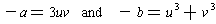
So, if we could find u and v so that these two equations were satisfied, then x = u + v would be the root of the cubic.
Now, compare these two equations to Lemma 3. It tells us that, in order to
make a quadratic with roots
 and
and
 , we just let the
first degree term be
, we just let the
first degree term be
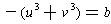 and the constant term be
 . So, the quadratic is
 Since we know how to solve every quadratic, we can find the roots of
this quadratic. If
Since we know how to solve every quadratic, we can find the roots of
this quadratic. If
 and
and
 are the two roots, then u and v are
simply the cube roots of these two roots, choosing them so that 3uv = -a.
But then x = u + v is a solution
to the original cubic and we have found a root of the cubic!
are the two roots, then u and v are
simply the cube roots of these two roots, choosing them so that 3uv = -a.
But then x = u + v is a solution
to the original cubic and we have found a root of the cubic!
By varying the cube roots, one expects to obtain the various solutions of the equation. But something is wrong here. We know that there are three cube roots and so pairing these up with each other, one expects to get 9 different pairs (u, v). But we know that a cubic has only 3 roots!
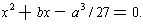
The problem is that we have created extraneous solutions. What we
did was to find pairs (u, v) so that
 . But our actual
equation was uv = -a/3. So, it is not enough to choose any pair of
cube roots of
. But our actual
equation was uv = -a/3. So, it is not enough to choose any pair of
cube roots of
 and
and
 . We need to choose the pairs so that uv = -a/3.
So, suppose our original pair was chosen so that uv = -a/3. If
 is a cube root of unity other than 1. Then the other cube roots of u
are
is a cube root of unity other than 1. Then the other cube roots of u
are
 and
and
 , and similarly for v. If we want another solution,
we can choose
, and similarly for v. If we want another solution,
we can choose
 for the new u. But then we must choose
 for the new v in order for the product to give the same value -a/3.
Similarly, if we choose
for the new v in order for the product to give the same value -a/3.
Similarly, if we choose
 for the new u, we have to choose
 for the v. So, we see that there are only three possible solutions
and not nine. This completes the solution of the general cubic.
for the v. So, we see that there are only three possible solutions
and not nine. This completes the solution of the general cubic.
Example 3:Solve the equation
 .
.
Our binomial expansion is
 .
Matching up with the original equation, we would want
.
Matching up with the original equation, we would want
 and
and
 . The quadratic that would
roots
. The quadratic that would
roots
 and
and
 is
is
 .
.
The quadratic factors as (x + 4)(x - 2) = 0. So the roots of the quadratic
are 2 and -4. Let u =
 and
and
 where we have
chosen the roots so that
uv = -2. One root is
where we have
chosen the roots so that
uv = -2. One root is
 .
To get the other roots, take a cube root of unity
.
To get the other roots, take a cube root of unity
 .
Then the other two roots will be
.
Then the other two roots will be
 and
and
 .
.
Example 4:Solve the equation
 .
Matching up with
.
Matching up with
 , gives 3uv = -1
and
, gives 3uv = -1
and
 .
The quadratic with
roots
.
The quadratic with
roots
 and
and
 would be
 .
.
The quadratic formula tells us that the roots of the quadratic are
 . One of the roots is positive and the second root is
negative. So, if you take the positive cube root of the positive one
and the negative cube root of the negative one, then their product will be
negative; so their sum will be one root. To get the other two roots,
first multiply one cube root by
. One of the roots is positive and the second root is
negative. So, if you take the positive cube root of the positive one
and the negative cube root of the negative one, then their product will be
negative; so their sum will be one root. To get the other two roots,
first multiply one cube root by
 and the other
by
and the other
by
 . Then multiply the first by
 and the second by
omega.
and the second by
omega.
3.5 Quartic Equations
Ferrari, a student of Cardan, showed that one could find the roots of the general quartic equation using techniques similar to those used for cubics. The story stops here. According to Abel's Theorem, there is no general formula for expressing the roots of a general polynomial equation of degree five or higher involving only arithmetic operations and roots.
Some fourth degree (quartic) polynomials are easy to solve. For example,
consider:
 . This can be factored

If the product is zero, then one factor or the other is zero. So, solving
for the roots of the quartic is the same as solving two quadratic equations,
which is something that one knows how to do. More generally, if we can arrange
the equation to be solved into the form:
 where p and q
are quadratic polynomials, then the roots are the roots of
where p and q
are quadratic polynomials, then the roots are the roots of
 and
and
 . As it will turn out, every fourth degree polynomial
can be put in this form.
. As it will turn out, every fourth degree polynomial
can be put in this form.
Let's start with a general fourth degree polynomial with complex number
coefficients. Dividing through by the leading coefficient, one needs to
solve an equation of the form
 . First, we can
assume that a = 0. In fact, if it were not, then one could apply the
same trick as we did with cubics. The first two terms look like the
first two terms of the expansion of
. First, we can
assume that a = 0. In fact, if it were not, then one could apply the
same trick as we did with cubics. The first two terms look like the
first two terms of the expansion of
 and so substituting x = y - a/4 converts our polynomial in x into one
in y with no cubic term. If one could solve the new polynomial in y, then
using x = y - a/4, one would get the roots of the original polynomial.
and so substituting x = y - a/4 converts our polynomial in x into one
in y with no cubic term. If one could solve the new polynomial in y, then
using x = y - a/4, one would get the roots of the original polynomial.
So, we can assume the form of the equation is:
 .
We can complete the square using the first two terms:
.
We can complete the square using the first two terms:
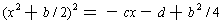 . We have one square on the left, we just
need to make the right side a square - but that is not promising because
the right side is only linear in x.
. We have one square on the left, we just
need to make the right side a square - but that is not promising because
the right side is only linear in x.
The problem is that we didn't quite choose the right constant term on the left side of the equation -- but how should we choose the right constant term? Since we don't know, we can simply adjust by adding y to the constant term. Our new equation becomes
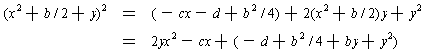
where we added the last two terms on the right in order to make the two
sides equal. Now, we have a square on the left and we need to choose y
so that we have a square on the right. But the right side is a quadratic
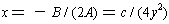
in x and so, we just need to make sure that this quadratic has both
roots equal. (If they were both equal to
 , then the right
side would factor as
, then the right
side would factor as
 as desired.) We need the following
result which is an obvious consequence of the quadratic formula:
as desired.) We need the following
result which is an obvious consequence of the quadratic formula:
Lemma 4: A quadratic
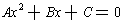 has two identical roots
precisely when
has two identical roots
precisely when
 .
.
Applying Lemma 4 to the right side of the equation, we see that we need y to satisfy:

But this is just a cubic equation in y. We can use the method of the
last section to find a y which satisfies this equation. Then, we
can factor the right side -- the roots are
 by the quadratic formula. So, our formula is just
Since both sides are squares, we see that we can find the roots of the quartic by solving two quadratics, viz.

This completes the solution of the general fourth degree polynomial equation.
All contents © copyright 2001 K. K. Kubota. All rights reserved